3 Basic energy models

In this chapter, we introduce the simplest climate model to describe the temperature of the Earth. Despite its apparent simplicity, this basic climate model is the foundation of all further discussion. We will find that, according to the most basic model, the surface temperature of the Earth is expected to be much colder than it is actually; we conclude that the likely culprit is greenhouse gases.

Consider the Earth as a single averaged body. Our goal is to obtain an equation for the surface temperature, $T$, by considering the energy recieved from the sun versus the energy the Earth must emit into space. This kind of balance-equation procedure is used everywhere in mathematical modelling. In essence, we are looking to write down a precise statement of the following:

Basic energy balance

\[ \text{Change in internal energy of Earth} = E_{\text{in}} - E_{\text{out}}, \tag{3.1}\]

where $E_{\text{in}}$ is the incoming energy from the sun and $E_{\text{out}}$ is the energy leaving the Earth. Note that the left hand-side (the internal energy) will depend on the temperature, $T$.

3.1 The basic energy model

The basic model is derived as follows.

By considering the incoming radiation from the sun, obtain an estimate for the incoming energy, $E_{\text{in}}$.
Use a constitutive law that indicates how much outgoing energy is produced by an object heated to some temperature.
Equate the change in internal energy to be equal to the difference between the above two items.

Note that the primary components of the global energy balance are radiative fluxes: we receive short-wave radiation (UV and visible light) from the Sun, and emit longwave radiation (infra-red) to space.

First we consider incoming energy.

Energy from the Sun

First, note that the shortwave radiation (UV and radiation) recieved from the sun is $Q \approx 1370 \text{ W$\cdot$m$^{-2}$}$ (which we consider measured at a point near the planet).

If we consider only that radiation that is absorbed into the Earth, we have \[ E_{\mathrm{in}} = \pi R^2 Q (1 - a), \tag{3.2}\] where $R$ is the Earth’s radius.

In the above formula, we have multiplied the flux, $Q$, with the visible surface area, $\pi R^2$. There is an additional multiplication by $(1 - a)$ where $a$ is the planetary albedo, which characterises amount of energy reflected due to the surface properties. Light surfaces like snow will have high albedo, $a \approx 0.9$, while darker surfaces like the ocean have smaller albedo, $a \approx 0.3$. The global average albedo is $a \approx 0.3$.

Next we consider outgoing energy.

Energy from the Earth

We now wish to characterise the energy, $E_{out}$, and in the case of Earth, this will correspond to longwave radiation (infra-red) emitted into space. All bodies characterised by a temperature, say $T_e$, will emit radiation, $Q_e$. As a model, we can consider $Q_e$ to be given by the Stefan-Boltzmann law, which states that \[ Q_e = \sigma T_e^4, \tag{3.3}\] where $\sigma \approx 5.67 \times 10^{-8} W m^{-2} K^{-4}$ is the Stefan-Boltzmann constant.

Now although the Earth’s surface may emit radiation according to (Equation 3.3), some of this radiation will be absorbed by the atmosphere and reflected back. This is the greenhouse effect. As a consequence of the greenhouse gas, the surface temperature of the Earth, $T$, will be larger than the effective emitting temperature, $T_e$. For the moment, we model this as \[ T_e = \gamma^{1/4} T_e, \tag{3.4}\] where $\gamma < 1$ is a greenhouse gas factor, which depends on the properties of the atmosphere.

Now combining the above equations, we have \[ E_{\mathrm{in}} - E_{\mathrm{out}} = \pi R^2 Q (1 - a) - 4\pi R^2 \sigma \gamma T^4, \tag{3.5}\] which gives the incoming energy per unit time.

Internal heat energy

Due to this incoming energy, the Earth will cool or heat in response. We need to know how the internal temperature of an object responds to an input in energy. The general formula is \[ \text{Internal heat energy} = \text{volume} \times (\rho c_p) \times T. \] The key quantity is the experimentally determined, $c_p$, which corresponds to the specific heat capacity. It is given in the SI units of $\mathrm{J} \cdot \mathrm{kg}^{-1} \cdot \mathrm{K}^{-1}$, i.e. energy per unit mass per unit temperature. Note that this applied to a shell around the planet of thickness $d$ in the atmosphere, and so the mass is given by \[ \text{mass} = (4 \pi R^2) d \rho \tag{3.6}\] where $\rho$ is the average density of the atmosphere. Let us imagine the increase in temperature, $\Delta T$,during an interval of time, $\Delta t$. You can now verify that \[ \Bigl[ (4 \pi R^2) d \rho \Bigr] c_p (\Delta T) \] returns the units of Joules—i.e. this is the internal energy produced during the time $\Delta t$. We then have \[ \Bigl[ (4 \pi R^2) d \rho \Bigr] c_p \Delta T = \Delta t (E_{in} - E_{out}). \]

Putting in (Equation 3.5) and taking the limit of $\Delta t \to 0$, we finally have a heat equation for the Earth’s temperature.

Zero-dimensional model for the surface temperature of the Earth

The Earth’s temperature, as measured on a layer of thickness $d$ at the troposphere is given by the following ordinary differential equation (ODE) for $T = T(t)$: \[ C \frac{\mathrm{d}T}{\mathrm{d}t} = \frac{1}{4} Q(1 - a) - \sigma \gamma T^4, \tag{3.7}\] where we have defined \[ C = \rho c_p d \] as the heat capacity of the atmosphere. Above, the solar flux, Q is often taken to be $Q = 1370$ W/m², $\sigma = 5.67 \times 10^{-8}$ W/(m²K⁴), and $\gamma \leq 1$ is the greenhouse gas factor.

The above equation Equation 3.7 is time-dependent, but we may consider that the surface temperature, either over long-time or in an averaged sense, is dictated by the steady-state (time-independent) solution. Setting $\mathrm{d}T/\mathrm{d}t$ to zero, we see that there is a unique steady-state given by \[ T = \left(\frac{Q(1-a)}{4\sigma\gamma}\right)^{1/4}. \]

If we take $Q \approx 1370 \,\mathrm{W m}^{-2}$, $a \approx 0.3$, $\sigma \approx 5.67 \times 10^{-8} \mathrm{W} \,\mathrm{m}^{-2} \mathrm{K}^{-4}$, we then get \[ T \approx 255 \mathrm{K} = -18^\circ \mathrm{C}. \] under the assumption that $\gamma = 1$. That’s pretty cold! The actual average temperature is around $288 \mathrm{K} \approx 15 ^\circ \mathrm{C}$.

The above back-of-the-envelope calculation seems to suggest that the parameter $\gamma < 1$ plays an important role in keeping the Earth warm enough for us to live on, and indeed the value of $\gamma$ inferred by the above is roughly $\gamma \approx 0.61$. Later on in the course, we will develop a more rigorous model to predict such a $\gamma$ by studying the properties of the atmosphere.

3.2 The history of global warming

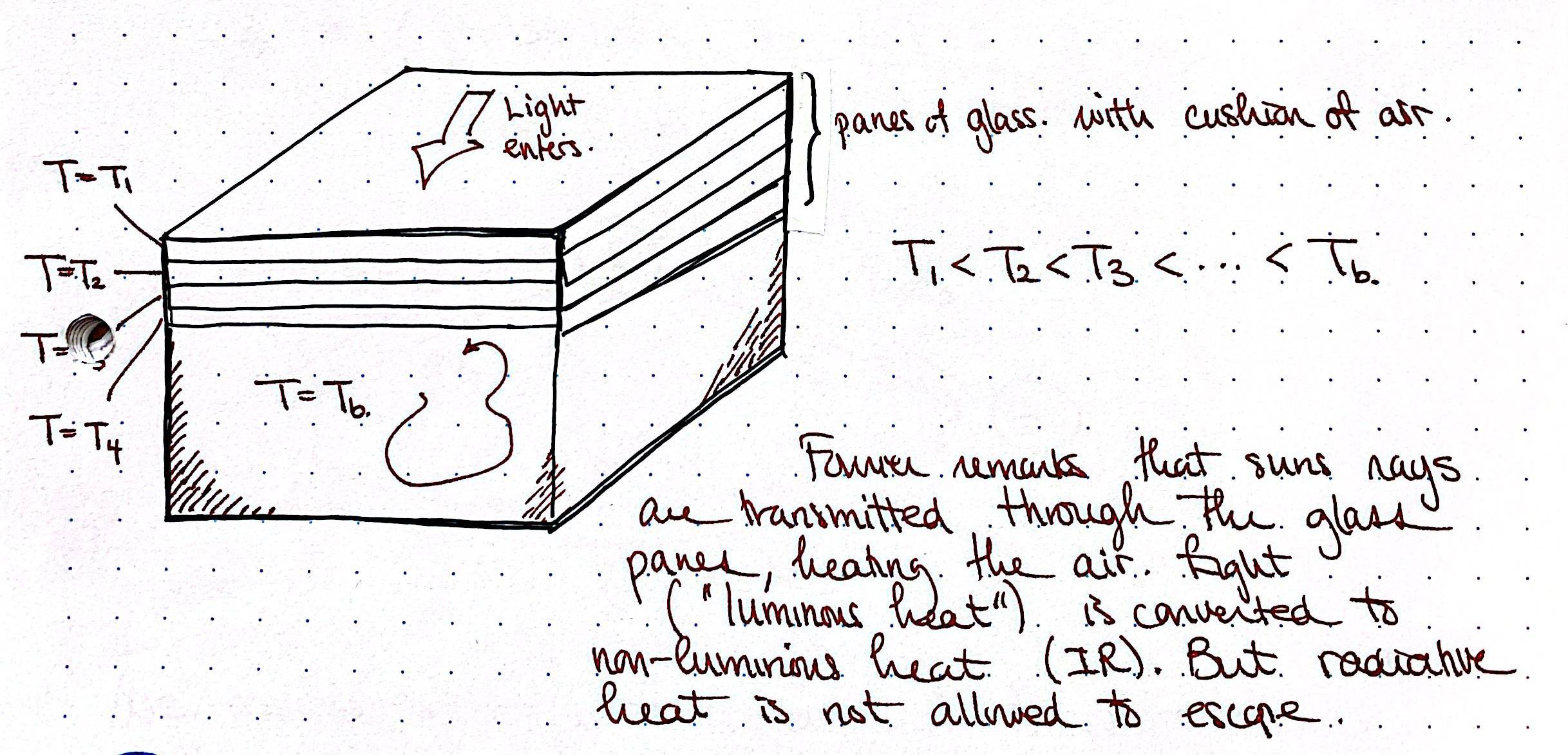
The history of global warming (and hence the estimation of $\gamma$) is convoluted, but the origins can be considered as far back as the work of (Fourier 1827) and (Pouillet 1838), and is discussed in the work by (Van der Veen 2000).

Figure 3.2: An illustration of Fourier’s glass box

3.3 Next in the study of energy balance models?

At this stage, the basic energy balance model studied in this chapter can be made more complex and realistic through many different extensions. For instance:

Consider the effects of a non-constant and nonlinear albedo. Since the albedo depends on the material property (water vs. ice vs. land), we can incorporate a toy model for spatial variability by allowing the albedo to depend on temperature, $a = a(T)$.
Consider the time-dependence. What happens if the system starts out of the steady state? Does it tend to relax to its equilibrium profile? Can we analyse the temporal properties of the solutions?
Can we incorporate latitude (or longitudinal) dependence into the model. For instance, should the albedo and solar radiation be considered as functions of the latitude?
Should we incorporate the effects of diffusion (heat spreading out) or convection (heat transported with flows)?
To what extent should we consider the effects of the atmosphere on the absorption and reflection properties of the incoming (and outgoing) energy?

Many of these questions are much more involve, as they require differential or partial differential equations. Therefore in the next few chapters, we will discuss, in a very general way, the collection of applied and numerical mathematics techniques that can be used when studying problems in the physical sciences.