6 Asymptotic approximations II

In the previous chapter, we learned about the technique of asymptotic expansions, whereby the solution of an equation is expressed in terms of a series in powers of a small parameter: \[ x = x_0 + \epsilon x_1 + \epsilon^2 x_2 + \ldots \] The precise choice of power progression (here integer powers of \(\epsilon\) will depend on the particular problem. The same idea can be extended to approximating solutions of differential equations. The upshot of this procedure is that at each order of the scheme, a simpler problem can be studied.

Again it is best to demonstrate through examples.

6.1 Returning to the projectile problem

In Chapter 4 and Chapter 26 you studied the non-dimensionalisation of the projectile problem. Once re-scaled, it takes the following form: \[ \begin{aligned} \frac{\mathrm{d}^2 y}{\mathrm{d}t^2} &= -\frac{1}{(1 + \epsilon y)^2}, \qquad t > 0 \\ y(0) &= 0, \\ y'(0) &= 1. \end{aligned} \tag{6.1}\]

This is a difficult problem without, in fact, any explicit solutions. However, we can estimate the solution in the limit \(\epsilon \to 0\). We expand the solution as \[ y(t) = y_0(t) + \epsilon y_1(t) + \epsilon^2 y_2(t) + \ldots \] In order to expand the denominator, you can use Taylor’s theorem to expand the function \[ f(x) = (1 + x)^\alpha = f(0) + f'(0)x + \ldots = 1 + \alpha x + \ldots \] around \(x = 0\).

The differential equation now yields \[ y_0'' + \epsilon y_1'' + \epsilon^2 y_2'' + \ldots = -\left[1 - 2\epsilon \left(y_0 + \epsilon y_1 + \ldots\right) + \ldots \right] \] so grouping terms together order-by-order yields \[ \Bigl[ y_0'' + 1 \Bigr] + \epsilon \Bigl[ y_1'' - 2y_0\Bigr] + \ldots = 0. \]

We can similarly substitute the expansion into the initial conditions. Altogether, at leading order, we obtain the following system to solve: \[ \begin{aligned} y_0'' + 1 &= 0, \\ y_0(0) &= 0, \\ y_0'(0) &= 1. \end{aligned} \] Integrating twice and applying the boundary conditions gives us \[ y_0(t) = -\frac{1}{2}t^2 + t. \] In fact, this is simply the parabolic motion you would expect from school Physics. The \(\epsilon = 0\) solution corresponds to assuming that the mass at the centre of the planet is dominant and then acceleration is constant.

However, we can now proceed to higher order and examine the nonlinear effects. Proceeding to \(O(\epsilon)\), we have the following system to solve: \[ \begin{aligned} y_1'' &= 2y_0, \\ y_1(0) &= 0, \\ y_1'(0) &= 0. \end{aligned} \] Notice the boundary conditions come from the fact there are no \(\epsilon\) corrections in the original boundary conditions, so \(y_n(0) = y_n'(0) = 0\) for all \(n > 0\). Again this system is simple to integrate. Integrating the solution for \(y_0\) twice and substitution of the initial conditions yields \[ y_1(t) = -\frac{1}{12}t^4 + \frac{1}{3}t^3. \] We have thus solved for the asymptotic approximation to two orders. We have \[ y(t) \sim \Bigl[ -\frac{1}{2}t^2 + t\Bigr] + \epsilon \Bigl[ -\frac{1}{12}t^4 + \frac{1}{3}t^3\Bigr]. \] This was quite an accomplishment! We have taken a problem that was not easily solvable in explicit form and through fairly simple integrations, obtained an approximation to two orders in \(\epsilon\). How good is it? Let us solve the problem numerically and compare with the asymptotic approximation.

6.2 Numerical solutions of IVPs

We first demonstrate how to solve ODEs (initial-value-problems, IVPs) using black-box functions in Python. For starters, most numerical formulations for ODEs will require that the problem be posed in terms of a first-order system of equations. To convert (Equation 6.1) into such a form, create a set of unknowns for the derivatives. Set \[ \mathbf{Y}(t) = \begin{pmatrix} y_1(t) \\ y_2(t) \end{pmatrix} = \begin{pmatrix} y(t) \\ y'(t) \end{pmatrix} \]

Then we have the following first-order system:

\[ \begin{aligned} \mathbf{Y}'(t) &= \mathbf{F}(t, \mathbf{Y}(t)) = \begin{pmatrix} y_1' \\ - \frac{1}{(1 + \epsilon y_1)^2} \end{pmatrix} \\ \mathbf{Y}(0) &= \begin{pmatrix} 0 \\ 1 \end{pmatrix} \end{aligned} \tag{6.2}\]

You can find a little guide on using solve_ivp in Python here. Here is the Python code to solve the differential equation.

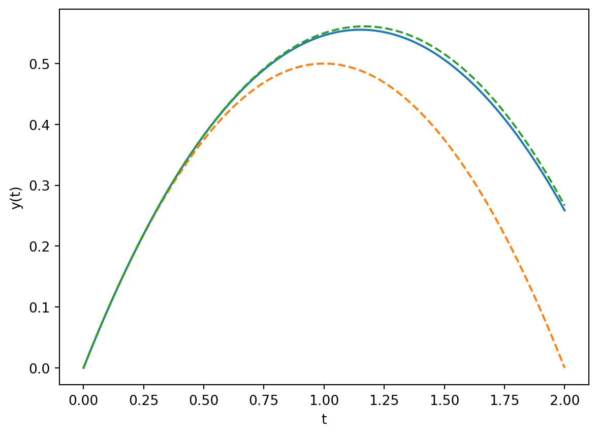
import numpy as np
import matplotlib.pyplot as plt
from scipy.integrate import solve_ivp

ep = 0.2 # epsilon value
tmax = 2 # max time
t = np.linspace(0, tmax, 100) # mesh used for plotting

# Define function for the ODE
def f(t, Y):
    ep = 0.2
    y, yp = Y
    ypp = -1/(1 + ep*y)**2
    return [yp, ypp]

# define the initial condition
Y0 = [0, 1]

sol = solve_ivp(f, [0, tmax], Y0, dense_output=True)

# Prior to plotting, re-interpolate solution on a fine grid
yy = sol.sol(t)
# Asymptotic solutions
y0 = -1/2*t**2 + t
y1 = -1/12*t**4 + 1/3*t**3

# Plot it all
plt.plot(t, yy[0,])
plt.plot(t, y0, '--')
plt.plot(t, y0 + ep*y1, '--')
plt.xlabel('t')
plt.ylabel('y(t)')

Text(0, 0.5, 'y(t)')

The two-term approximation does beautifully well, even at this moderate value of \(\epsilon = 0.2\).