7  Numerical solutions of IVPs

In the previous section, we used built-in ODE solvers to develop numerical solutions. It is important to gain an understanding how a simple ODE solver works. The simplest scheme is called Euler’s method, and this we now explain.

Begin from the system (Equation 6.2). We assume that the solution is represented by a discrete set of points, \(\mathbf{Y}_n = \mathbf{Y}(t_n)\) at the times \(t_0 = 0\), \(t_1 = \Delta t\), \(t_2 = 2\Delta t\), and so on. The time derivative is written as a discrete derivative while we approximate the right hand side by its value at the nth time step: \[ \frac{\mathbf{Y}_{n+1} - \mathbf{Y}_{n}}{\Delta t} = \mathbf{F}(t_n, \mathbf{Y}_n) \]

Rearranging yields a very simple algorithm for solving the ODE: \[ \mathbf{Y}_{n} = \mathbf{Y}_{n-1} + \mathbf{F}(t_{n-1}, \mathbf{Y}_{n-1}) \Delta t \] for \(n = 1, 2, 3, \ldots\)

This would be implemented via the following pseudocode:

Euler’s method

1. Input: function f(t, Y)  
            time step, dt
            initial condition, Y0

2. Set initial condition Y = Y0

2. Take one Euler step and overwrite previous value

                 Y = Y + f(t, Y)

3. Increment t by dt and goto 2

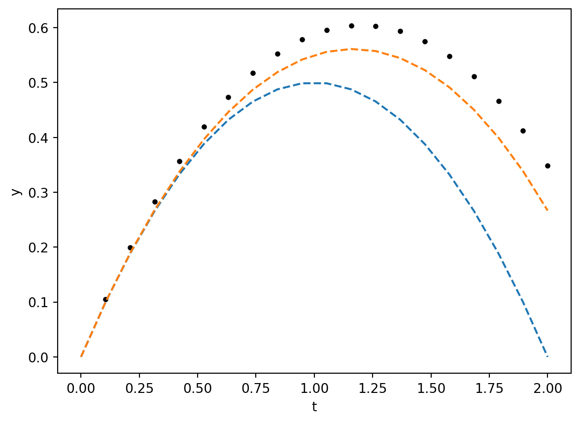
Euler’s method is conceptually simple but quite inaccurate. But in this case, we see that it works fairly well in comparison to the built-in solvers.

import numpy as np
import matplotlib.pyplot as plt
from scipy.integrate import solve_ivp

ep = 0.2            # epsilon value
tmax = 2            # max time
N = 20              # number of steps
t = np.linspace(0, tmax, N) # mesh used for plotting
dt = t[1] - t[0]

# Define function for the ODE
def f(t, Y, ep):
    y, yp = Y
    ypp = -1/(1 + ep*y)**2
    return np.array([yp, ypp])

# define the initial condition
Y = [0.0, 1.0]
ti = 0

# define the solution vector
for i in range(1, N):
    ti = ti + dt  # Increment time
    Y = Y + f(ti, Y, ep)*dt # Euler step
    plt.plot(ti, Y[0], 'k.')

# Asymptotic solutions
y0 = -1/2*t**2 + t
y1 = -1/12*t**4 + 1/3*t**3
plt.plot(t, y0, '--')
plt.plot(t, y0 + ep*y1, '--')
plt.xlabel('t');
plt.ylabel('y');