In Chapter 6, we studied how asymptotic expansions can be used to approximate equations like \[
\frac{\mathrm{d}^2 y}{\mathrm{d}t^2} = -\frac{1}{(1 + \epsilon y)^2}
\] by expanding the solution as \(y(t) = y_0(t) + \epsilon y_1(t) + \ldots\). These are known as regular problems because a small perturbation, \(\epsilon\), does not seem to fundamentally change the \(\epsilon = 0\) solution beyond a small perturbation. This is not always the case. In singular problems, the situation of \(\epsilon \neq 0\) is fundamentally different than the situation from \(\epsilon = 0\). You have already seen such an example in Chapter 5. The equation \[
\epsilon x^2 + x - 1 = 0
\] has one root for \(\epsilon = 0\) and two roots for non-zero small \(\epsilon\)—even infinitesimally small values! This is quite interesting. From a wider scientific perspective, you may wonder what other problems in nature possess such singular effects.
The point of this lecture is study a technique known as matched asymptotics. These matched asymptotics are often necessary for singularly perturbed differential equations.
8.2 A singular first-order ODE problem
\(\nextSection\)
Previously in Chapter 4, we derived a basic equation that governs the temperature on the surface of the planet. This equation had the following form: \[
(\rho c_p V) \frac{\mathrm{d}T}{\mathrm{d}t} = E_{\text{in}}(t, T) - E_{\text{out}}(t, T).
\]
For the purpose of this section, let us make up a toy model. We suggest, in non-dimensional form, \[
\begin{aligned}
\epsilon \frac{\mathrm{d}T}{\mathrm{d}t} &= R(t) - T, \quad t \geq 0 \\
T(0) &= T^*,
\end{aligned}
\tag{8.1}\] where we consider \(\epsilon > 0\) and \(\epsilon \ll 1\). You can think of the above model as modelling the temperature on a substance that radiates heat in a fashion proportional to itself (\(-T\)) and is being subjected to an (incoming) heat source, \(R\). Let us take as an example, \[
R(t) = 1 + A \cos(t).
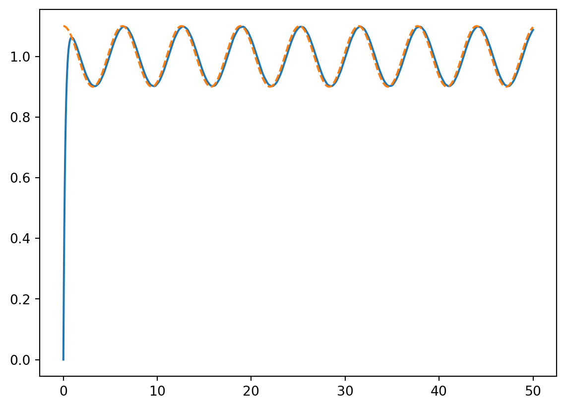
\] Our choice for \(R\) is not so important. This equation is, in fact, solvable in closed form (how?) but let us get additional practice solving numerically.
What do we observe? If \(\epsilon = 0\), then we expect the solution \(T \sim R(t)\). This is shown with the dashed line. However, this solution does not satisfy the necessary initial condition. We observe that near \(t = 0\), the exact solution seems to very rapidly diverge from the approximation in order to satisfy the proper boundary condition. The region in \(t\) where this rapid change occurs is called a boundary layer.
If we repeat the experiment with an even smaller value of \(\epsilon\), we would observe that the size of this boundary layer seems to tends to zero as \(\epsilon \to 0\). This numerical experiment thus inspires the following method.
8.3 Boundary layer theory
\(\nextSection\)
We seek a method that will allow us to develop a uniformly valid approximation, i.e. an approximation that is good everywhere in the relevant domain, \(t \geq 0\). Begin by performing the usual asymptotic approximation: \[
T(t) = T_0(t) + \epsilon T_1(t) + \epsilon^2 T_2(t) + \ldots
\] Substitution into the ODE (Equation 8.1) yields at leading order, \[
0 = R(t) - T_0(t) \Longrightarrow T_0(t) = R(t) = 1 + A \cos(t).
\] As we have noted, this approximation fails to satisfy the initial condition, \(T(0) = T^*\) in general. It is possible to go to higher order but this is not so important at the moment. So for now, we have obtained: \[
T_{\text{outer}} \sim \Bigl[ 1 + A\cos t\Bigr].
\] We have chosen to refer to this as the outer solution for reasons that will be abundantly clear. But rather than satisfying \(T(0) = T^*\), this approximation has the limiting behaviour of \[
\lim_{t \to 0} T_{\text{outer}} \sim \Bigl[ 1 + A\Bigr]
\] Above, we have only included the leading term in the limit expression.
8.3.1 The inner scaling
\(\nextSection\)
Our intuition follows a very similar logic to the examination of the singular root in Section 5.1.1. Above, our naive assumption was that \(\epsilon T'(t)\) could be ignored since \(\epsilon\) is a small number. However, this may not be the case if the gradient is very large.
Our intuition further suggests that the boundary layer occurs near \(t = 0\) and that it scales in size with \(\epsilon\). Therefore, let us set \[
t = \epsilon^{\alpha} s,
\] as a change of coordinates. We expect \(\alpha > 0\) (otherwise \(t\) is not small), and within this region, we expect the new coordinate, \(s\), to be \(O(1)\) (of moderate size). We then transform the unknown function: \[
T(t) = T(\epsilon s) = U(s),
\] and seek a new differential equation for \(U\). By the chain rule, \[
\frac{\mathrm{d}T}{\mathrm{d}t} = \epsilon^{-\alpha} \frac{\mathrm{d}U}{\mathrm{d}s}.
\] Before substituting into the equation, we are prudent to examine the behaviour of \(R(t)\) near \(t = 0\). We know by Taylor’s theorem that \[
R(t) = 1 + A \left(1 - \frac{t^2}{2} + \ldots \right).
\] Therefore, under the substitution, we may approximate \(R\) by its leading terms: \[
R( \epsilon^{\alpha} s) \sim 1 + A.
\] For now, we will not need more terms than this. Substituting into the ODE now gives \[
\epsilon^{1-\alpha} \frac{\mathrm{d}U}{\mathrm{d}s} \sim \Bigl[1 + A\Bigr] - U.
\] Now in order to involve the first term, it is sensible to select \[
1 - \alpha = 0 \Longrightarrow \alpha = 1.
\]
8.3.2 The inner equation
\(\nextSection\)
Therefore, the correct coordinate re-scaling was the ‘obvious’ one: \[
t = \epsilon s.
\]
Substituting this again in (Equation 8.1): \[
\begin{aligned}
\frac{\mathrm{d}U}{\mathrm{d}s} &= 1 + A\cos(\epsilon s) - U, \\
U(0) &= T^*.
\end{aligned}
\]
The procedure is now exactly the same. We expand \[
U(s) = U_0(s) + \epsilon U_1(s) + \epsilon^2 U_2(s) + \ldots
\] At leading order, we get \[
\begin{aligned}
U_0' &= 1 + A - U_0 \\
U_0(0) &= T^*.
\end{aligned}
\]
The above ODE can be solved by integrating factors. Multiplying both sides be \(e^s\), we have \[
(U_0 e^s)' = (1 + A)e^s.
\] Integrate and use the initial condition: \[
U_0(s) = (1 + A) + (T^* - (1 +A))e^{-s}.
\] This is exactly what we expect. Notice that \[
\lim_{s \to \infty} U_0(s) = \lim_{t \to 0} T_{\text{outer}}
\tag{8.2}\] therefore the outer limit of our inner solution matches the inner limit of our outer solution. In terms of outer coordinates, our inner solution is approximated as follows: \[
T_{\text{inner}} \sim (1 + A) + (T^* - (1 +A))e^{-t/\epsilon}.
\]
Let us summarise the procedure of matched asymptotics.
Expand the solution of the differential equation naively in the typical asymptotic expansion (e.g. in powers of \(\epsilon\)).
Notice that the approximation does not satisfy certain boundary conditions.
Re-scale the coordinates in the ‘inner’ regions.
Develop an inner solution that satisfies the boundary condition. Ensure it matches the outer solution.
You will get more practice of this procedure in the problem sets.
8.3.4 An additional problem
\(\nextSection\)
In Lecture 8 (26 Feb 2025), problem class, and associated problem set, we studied the example of \[\begin{gather}
\epsilon T'' + 2T' + T = 0, \qquad t \in [0, 1], \\
T(0) = 0, \qquad T(1) = 1.
\end{gather}\]
This is an example where the inner solution, near \(t = 0\), requires the solution of a second-order differential equation that requires matching to the outer solution. You can follow the matching procedure via the visualiser notes (and it is further touched-upon in the problem set).