38 Problem set 6 solutions

Q1. A van der Pol equation

Determine $f(x)$ so that this equation can be written as a Liénard phase plane system in the form \[ \begin{aligned} \epsilon \dot{x} &= f(x) + 4y, \\ \dot{y} &= -x. \end{aligned} \]

Solution

Start from the ODE and re-write \[ \frac{\mathrm{d}}{\mathrm{d}t} \left[\epsilon \dot{x} + (x^3 - 3x^2 - 9x)\right] = - 4x. \] Double check that the derivative of the LHS returns the original problem. Now set the quantity in brackets equal to one unknown: \[ \tilde{y} = \epsilon \dot{x} + (x^3 - 3x^2 - 9x), \] and solve for the derivative: \[ \epsilon \dot{x} = \tilde{y} - (x^3 - 3x^2 - 9x). \] The remaining equation is \[ \dot{\tilde{y}} = -4x. \]

Now in this question, we have chosen a slightly different choice to eliminate the factor of $4$. Set $\tilde{y} = 4y$ to get the system

\[\begin{align} \epsilon \dot{x} &= f(x) + 4y, \\ \dot{y} &= -x. \end{align}\]

It doesn’t really matter which choice you select. So here we see $f(x) = -x^3 + 9x + 3 x^2$. What we often call the slow manifold in lectures is then \[ y = -f(x)/4 = \frac{x^3 - 3 x^2 - 9x}{4} \equiv S(x). \]

For fixed $\epsilon > 0$, find the equilibrium point(s) in the phase plane, find their eigenvalues, and classify their linear stability.

Solution

The only equilibrium point is $(x_*, y_*) = (0,0)$. Because the equilibrium point is at the origin, we can obtain the linear matrix by ignoring the higher-order powers in the differential equations. The matrix is \[ A = \begin{pmatrix} \frac{9}{\epsilon} & \frac{4}{\epsilon} \\ -1 & 0 \end{pmatrix}. \] Subtract $\lambda$ from the diagonal elements and solve the resultant quadratic equation $\lambda(\lambda - 9/\epsilon) + 4/\epsilon = 0$ to see that the eigenvalues are $\lambda = (9 \pm \sqrt{81 - 16\epsilon}/(2\epsilon) > 0$, so the point is an unstable node.

Use the expansions $x(t) = x_0(t) + \epsilon x_1(t) + O(\epsilon^2)$ to determine the equations for the leading-order slow solution. Sketch the slow manifold, indicate the directions motion on each part, and identify the two attracting points on the curve.

Solution

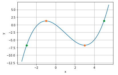
As usual expand the solutions into a series in powers of $\epsilon$. The slow manifold is $y_0(x_0) = S(x_0) = (x_0^3 - 3 x_0^2 - 9 x_0)/4$. In image of the slow manifold is shown below in blue. Notice that for $x < 0$, $y$ is increasing and for $x > 0$, $y$ is decreasing (due to the second differential equation).

Figure 38.1: Illustration of slow manifold

Use the expansions $x(t) = X_0(T) + \epsilon X_1(T) + O(\epsilon^2)$ and $y(t) = Y_0(T) + \epsilon Y_1(T) + O(\epsilon^2)$ with $T = t/\epsilon$ to obtain the leading-order fast solution.

Solution

Rescale $t = \epsilon T$ and re-write $x = X(T)$ and $y = Y(T)$. We get \[ \begin{align} \frac{\mathrm{d}X}{\mathrm{d}T} &= f(X) + 4Y \\ \frac{\mathrm{d}Y}{\mathrm{d}T} &= -\epsilon X. \end{align} \]

Now expand into powers of $\epsilon$ and take the leading-order: \[ \begin{align} \frac{\mathrm{d}X_0}{\mathrm{d}T} &= f(X_0) + 4Y_0 \\ \frac{\mathrm{d}Y_0}{\mathrm{d}T} &= 0. \end{align} \]

The second equation indicates that $Y_0$ is constant. Its value, found in part (e) is either $5/4$ or $27/4$. The remaining equation for $X_0$ is nonlinear and there is not much you can do with it. The important item of understanding is to examine its form: \[ \frac{\mathrm{d}X_0}{\mathrm{d}T} = f(X_0) + 4 Y_0. \] Now on the upper branch of the picture shown above $f(X_0) = 4 Y_0 > 0$ and therefore the solution increases its value in $X_0$ until it intersects with the blue slow manifold, at which point its rate of change is zero and it descends the slow manifold. A similar behaviour occurs on the lower branch of the fast evolution.

Use the phase plane to determine the maximum and minimum values of $x(t)$ during an oscillation. Sketch $x(t)$ as a function of time.

Solution

By checking the derivatives, we can see that the slow manifold has local extrema at $(-1, 5/4)$ and $(3, 27/4)$. In the fast evolution stages, $y$ is constant and $x$ evolves from one extrema value to the other on the slow manifold, satisfying $y = S(x)$.

Here is a plot of the key points.

Q2. Fast-slow dynamics with three variables

For the system \[ \begin{aligned}[c] \dot{x} &= 2 - y, \\ \dot{y} &= x-z, \\ \epsilon\dot{z} &= y - y^2 + \frac{1}{3}y^3 - z, \end{aligned} \] with the initial conditions of $x(0) = 1$, $y(0) = 3$, and $z(0) = 0$.

Identify the surface $z = S(x, y)$ that defines the slow manifold. Find the equilibrium point of the leading=order slow phase plane system and show that it is asymptotically stable for $t \to \infty$. Also determine the form of the initial layer that describes the transition from the initial conditions to the slow manifold.

Solution

Setting $\epsilon = 0$ we see that the slwo manifold is $z = S(y) = y - y^2 + y^3/3$. The leading-order slow system is

\[\begin{align} \frac{\mathrm{d}x_0}{\mathrm{d}t} &= 2 - y_0 \\ \frac{\mathrm{d}y_0}{\mathrm{d}t} &= x_0 - y_0 + y_0^2 - y_0^3/3. \end{align}\] $$ The only equilibrium point is $(x^*, y^*) = (2/3, 2)$. Linearisation gives eigenvalues of $\lambda = 1/2(-1 \pm 3i)$ so the point is a stable spiral. Consequently the $t \to \infty$ solution will be $(x, y, z) = (2/3, 2, 2/3)$. Note also that $2/3 = S(2)$.

Near the initial condition there is a boundary layer, found by setting \[ t = \epsilon T, \] and transforming $x = X(T)$, $y = Y(T)$, $z = Z(T)$. We get at leading order,

\[\begin{align} \frac{\mathrm{d}X_0}{\mathrm{d}T} &= 0 \\ \frac{\mathrm{d}T_0}{\mathrm{d}T} &= 0 \\ \frac{\mathrm{d}Z_0}{\mathrm{d}T} &= Y_0 - Y_0^2 + Y_0^3/3 - Z_0. \end{align}\]

The initial condition sets $X_0 = 1$ and $Y_0 = 3$. We can finally solve the equation for $Z_0$ to get \[ Z_0 = 3(1 - e^{-T}). \]

For the system \[ \begin{aligned}[c] \dot{x} &= 2 - y, \\ \epsilon\dot{y} &= x-z, \\ \dot{z} &= y - y^2 + \frac{1}{3}y^3 - z, \end{aligned} \] with the initial conditions of $x(0) = 0$, $y(0) = 3$, and $z(0) = 1$.

Show that the slow manifold reduces to a curve that could be written in parametric form as $x = x(z), y = y(z), z = z$. Determine the asymptotic solution for $t \to \infty$. Also determine the form of the initial layer that describes the transition from initial conditions to the slow manifold.

Solution

Setting $\epsilon = 0$, we see that the second equation gives $x = z$. Now if you use this result in the first equation you obtain $\dot{z} = 2 - y$. This is now equated with the third equation which yields an algebraic equation: \[ 2 - y = y - y^2 + \frac{y^3}{3} - z \Longrightarrow z = \frac{y^3}{3} - y^2 + 2y - 2. \tag{38.1}\] Therefore we conclude that $z = z(y)$. We can verify that this equation is monotonically increasing in $y$, so we can invert without issue, yielding $y = y(z)$. Similarly, we obtain $x = z$. So the slow manifold is given by \[ (x, y, z) = (z, y(z), z), \] which is a curve in 3D.

In order to determine what happens as $t\to\infty$, differentiate \[ \frac{\mathrm{d}y}{\mathrm{d}t} = \frac{\mathrm{d}y}{\mathrm{d}z} \frac{\mathrm{d}z}{\mathrm{d}t} = \frac{2 - y}{2 - 2y + y^2}, \] which follows from using the first equation of the system of ODEs and also the $z$ derivative of (Equation 38.1). In particular, note that we do not have to invert this latter equation and we can take the $y$-derivative of (eq-PS5-Q3-tmp) and use \[ \frac{1}{\frac{\mathrm{d}z}{\mathrm{d}y}} = \frac{1}{2 - 2y + y^2}. \]

Take $dy/dt = 0$ for the steady state gives \[ y^* = 2, \] as the only fixed point. At this value of $y$, notice that $z^* = 2/3$ from (Equation 38.1). So the fixed point is \[ (x^*, y^*, z^*) = (2/3, 2, 2/3). \]

The procedure for the initial layer is the same as in part (a). This time, the fast system satisfies at leading order,

\[\begin{align} \frac{\mathrm{d}X_0}{\mathrm{d}T} &= 0 \\ \frac{\mathrm{d}Y_0}{\mathrm{d}T} &= X - Z \\ \frac{\mathrm{d}Z_0}{\mathrm{d}T} &= 0. \end{align}\]

So we obtain $X_0 = 0$ and $Z_0 = 1$ using the initial condition. Solving for the final equation for $Y_0$ with $Y_0(0) = 3$ gives \[ Y_0 = -T + 3. \]