21 Basic models of the ocean
21.1 Terminology and context
The ocean plays a significant role in regulating the Earth’s climate, as it acts as a massive heat sink and helps to distribute heat and moisture around the planet. In addition, carbon dioxide is water soluble, and through precipitation and wave motion, is transferred into the oceans. Thus the ocean acts as a sink, absorbing large amounts of this greenhouse gas from the atmosphere.
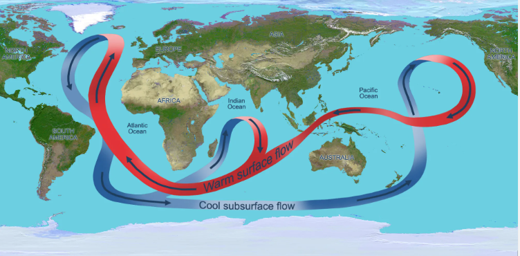
The thermohaline circulation (THC), also known as the global ocean conveyor belt, is a complex ocean circulation pattern that is driven by differences in water temperature and salinity. It is an important component of the Earth’s climate system, as it helps to distribute heat and other properties throughout the planet’s oceans.
The thermohaline circulation is driven by the sinking of cold, dense water in the polar regions, which then spreads out and flows towards the equator. As the water warms and becomes less dense, it rises to the surface and returns to the poles, creating a continuous loop of ocean currents. The role of salinity in driving the thermohaline circulation is due to the fact that the dissolved salts in seawater increase its density.
This circulation pattern has a significant impact on global climate, as it helps to regulate the exchange of heat and other properties between the oceans and the atmosphere. Changes in the thermohaline circulation, such as those caused by global warming, can have far-reaching effects on the planet’s climate and weather patterns.
21.2 Temperature
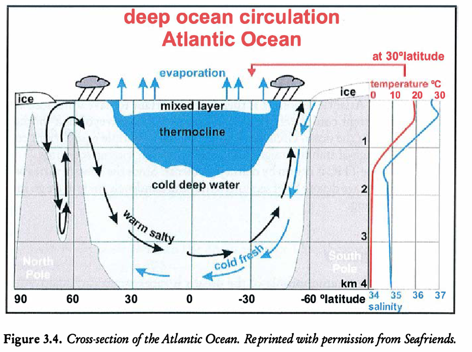
In regards to the temperature, the ocean can be divided into three layers.
The top layer is thin (on the order of metres) and is heated from the Sun. Mixing is a dominant effect due to wind and waves, and so the temperature in this region is mostly constant.
The thermocline region is the intermediate layer. Here, the temperature decreaes approximately linearly.
The deep abyssal zone comprises 98% of the total volume of the oceans. The temperature in this region is mostly constant, and a few degrees above freezing.
Within the intermediate region, the temperature can be modelled by an advection diffusion equation, \[ \frac{\mathrm{\partial}T}{\mathrm{\partial}t} + w \frac{\mathrm{\partial}T}{\mathrm{\partial}z} = \kappa \frac{\mathrm{\partial}^2 T}{\mathrm{\partial}z^2}, \tag{21.1}\] where \(w\) is the upswelling velocity and \(\kappa\) is the diffusion coefficient of the fluid.
Let us assume that the temperature in this region is near steady state and that the upwards velocity is constant. Then we integrate the ODE to find \[ T(z) = T_0 + T_1 \mathrm{e}^{-z/z^*}, \] where \(T_0\) and \(T_1\) are constants. From (Kaper and Engler 2013), the typical orders for the parameters are \(\kappa \sim 10^{-2} \,\mathrm{m}^{2} \,\mathrm{s}^{-1}\) and \(z^* \sim 10^2 \, \mathrm{m}\), so \(w \sim 10^{-4} \,\mathrm{m} \,\mathrm{s}^{-1}\), which is quite slow.
21.3 Salinity and density
Salinity is a key component in the oceans since the salts have a large effect on the water density (which consequently drives motion). Salinity is measured in psu or practical salinity units, which is a non-dimensional ratio of conductivities. In the mixed layer, the sainity ranges from 31-39 psu, and is about 35 in the abyssal zone. You can inspect the profile in Figure 21.2.
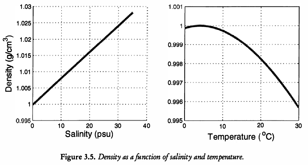
Below in the study of the ocean, we will need a so-called equation of state, which connects the density, \(\rho\), with the salinity, say \(S\), and temperature, say \(T\). Here is a typical graph of the relationship.
21.4 Two-box model of the ocean
Modelling the THC is a challenging task! In principal, this might involve the solution of multiple coupled PDEs for the flows and temperatures, which would then need to be solved on a very complicated domain. In addition, such models require a number of empirical equations of state (connecting density to temperature and salinity).
Toy models can be developed much more easily at the ‘systems level’ via box models.
21.5 A one-dimensional model (constant temperature)
Construction and assumptions of the box model.
We consider two boxes, labeled ‘1’ and ‘2’, respectively via subscripts. Box 1 corresponds to high latitudes (near poles) and Box 2 to low latitudes (near equator). Each box has a corresponding temperature, \(T_i\), and salinity, \(S_i\). In each box, the temperature and salinities are well mixed, so they take different values in either box, in general.
Differences between the two boxes will drive a flow through the capillary pipe that connects the boxes at the bottom. A compensating flow at the surface ensures that the volume of water in each box does not change. Together, these two exchanges (top and bottom) represent the overturning circulation of the THC.
We assume (see above) that the strength of the exchange flow between the boxes is linearly proportional to their differences of temperature and salinity. In particular, let \(\rho_1\) and \(\rho_2\) be the two densities in the corresponding boxes. The flow \(q\) in the capillary pipe is driven by the difference \[ q = k \frac{\rho_1 - \rho_2}{\rho_0}, \tag{21.2}\] where \(k\) is the hydraulic constant and takes the typical value of \(k = 1.5 \cdot 10^{-6} \, \mathrm{s}^{-1}\). The reference density \(\rho_0\) is defined in conjunction with the equation of state.
In the normal state of the planet, \(q > 0\) when the flow through the capillary goes in the direction of the equator as a result of higher densities at high latitudes.
We need an equation of state that connects the densities, \(\rho\), with the temperature and salinities. This concerns the figure Figure 21.3. We assume that \[ \rho = \rho_0(1 - \alpha(T - T_0) + \beta(S - S_0)), \tag{21.3}\] where \(T_0\) and \(S_0\) are average values of temperature and salinity; \(\rho_0\) is the density if \(T = T_0\) and \(S = S_0\); \(\alpha\) and \(\beta\) are constants with typical values \(\alpha = 1.5 \times 10^{-4} \mathrm{deg}^{-1}\) and \(\beta = 8 \times 10^{-4} \mathrm{psu}^{-1}\). Combining (Equation 21.2) with (Equation 21.3) gives \[ q = k[ \alpha(T_2 - T_1) - \beta(S_2 - S_1)]. \tag{21.4}\]
External wind forces and Coriolis effects are ignored.
We assume that in each box, there is an exchange of heat and salinity to the surrounding environment. For instance, salinity will exchange due to evaporation, precipitation, and runoff. These will have constant of proportionalities of \(c\) and \(d\) in the equations below.
Precipitation, evaporation, and runoff from the continents and atmosphere will also cause the salinity in either box to change. We therefore assume that this is modeled by a flux \(H\).
Remember that in general, \(T_2 > T_1\) (the temperatures at the equator are higher). Consequently, evaporation dominates Box 2; there is a net loss of salt-free moisture in the atmosphere and this causes a compensating virtual flux of salt, \(H > 0\), into Box 2. At the same time, there is higher precipitation and runoff into Box 1 (due to lower temperatures), causing a net gain of salt-free moisture and therefore a loss of virtual salt, say \(-H < 0\). We assume these two virtual salt fluxes sum to zero.
Note that in the normal state of affairs, \(S_2 > S_1\), and the lower latitude water is saltier than that of high latitudes.
An image of the box model is shown below.
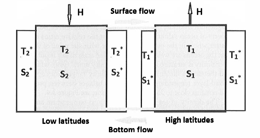
The equations are given as follows. \[ \begin{aligned} \frac{\mathrm{d}T_1}{\mathrm{d}t} &= c(T_1^* - T_1) + |q|(T_2 - T_1) \\ \frac{\mathrm{d}T_2}{\mathrm{d}t} &= c(T_2^* - T_2) + |q|(T_1 - T_2) \\ \frac{\mathrm{d}S_1}{\mathrm{d}t} &= -H + d(S_1^* - S_1) + |q|(S_2 - S_1) \\ \frac{\mathrm{d}S_2}{\mathrm{d}t} &= H + d(S_2^* - S_2) + |q|(S_1 - S_2) \end{aligned} \tag{21.5}\]
Note that in the exchange terms corresponding to the flow \(q\) in the capillary pipes, we use an absolute value since it does not matter (flows are exchanged in both lower and upper pipes).
Note also that \(q = q(T_1, T_2, S_1, S_2)\) as given in (Equation 21.4).
21.6 Reducing the equations via symmetry
By adding the equations (Equation 21.5), it can be verified that in the limit \(t \to \infty\), the average temperature in the system, \(1/2(T_1 + T_2)\) tends to the average temperature in the surrounding basins \(1/2(T_1^* + T_2^*)\). The same conclusion can be drawn for the corresponding salinities.
It is then sensible to write all temperature and salinity in terms of this baseline scenario. So let us write \[ \begin{aligned} T_1 &= \frac{1}{2}m + U_1, \\ T_2 &= \frac{1}{2}m + U_2, \end{aligned} \] where \(m = T_1^* + T_2^*\). Then the first equation becomes \[ \begin{aligned} \frac{\mathrm{d}U_1}{\mathrm{d}t} &= c\left(T_1^* - U_1 - \frac{1}{2}m\right) + |q| (U_2 - U_1)\\ &= c\left(- T^* - U_1\right) + |q| (U_2 - U_1). \end{aligned} \] where \(T^* = \frac{1}{2}(T_2^* - T_1^*)\).
The analogous manipulations are done to the quantities for the salinity. In the end, if we (confusingly) re-write \(T\) for \(U\), then we obtain \[ \begin{aligned} \frac{\mathrm{d}T_1}{\mathrm{d}t} &= c(-T^* - T_1) + |q|(T_2 - T_1) \\ \frac{\mathrm{d}T_2}{\mathrm{d}t} &= c(T^* - T_2) + |q|(T_1 - T_2) \\ \frac{\mathrm{d}S_1}{\mathrm{d}t} &= -H + d(-S^* - S_1) + |q|(S_2 - S_1) \\ \frac{\mathrm{d}S_2}{\mathrm{d}t} &= H + d(S^* - S_2) + |q|(S_1 - S_2) \end{aligned} \tag{21.6}\]
Comparing the above to Equation 21.5, the main difference is that, in expressing the temperature and salinities with respect to the average values in the basin, we have eliminated two of the constants from the set \((T_1^*, T_1^*, S_1^*, S_2^*)\) now only into two constants \((T^*, S^*)\).
In the situation of zero salt flux. \(H = 0\), the above model reduces to Stommel’s box model studied later in this course.
21.7 Analysis of a reduced 1D model for the salinity
It is possible to do some analysis on the system (Equation 21.6), though we may prefer to simply move on to study the more historically well-known reduction called Stommel’s box model.
We make the following assumptions:
- We assume that on the timescale of interest in the THC, the temperature of each box equilibrates quickly with the surrounding basin. Therefore the system can be regarded as being in steady state.
- The difference in temperatures between the two boxes is small; together with the top assumption, this implies that \(T_1(t) = -T^*\) and \(T_2(t) = T^*\).
- Salinity exchanges by negligible amounts with its surrounding basin, i.e. \(d = 0\)
This leaves us with \[\begin{align*} \frac{\mathrm{d}S_1}{\mathrm{d}t} &= -H + |q|(S_2 - S_1) \\ \frac{\mathrm{d}S_2}{\mathrm{d}t} &= H + |q| (S_1 - S_2), \end{align*}\] where \(q = k(2\alpha T^* - \beta(S_2 - S_1))\).
Now, the formulation for the salinities can be placed into a single equation for \(\Delta S = S_2 - S_1\), which satisfies \[ \frac{\mathrm{d}\Delta S}{\mathrm{d}t} = 2H - 2k|\alpha \Delta T - \beta \Delta S| \Delta S. \tag{21.7}\]
This is now a much simpler and elegant formulation for study. Under a suitable non-dimensionalisation and scaling, we can even place the above equation in the final simplified form of \[ \dot{x} = \lambda - |1 - x| x, \] where \(\lambda > 0\) (for temperatures in the usual configuration, with \(T_2 - T_1 > 0\), and a suitably defined function \(x = x(t)\).