34 Problem set 2 solutions

34.1 Getting started with Jupyter

Note

N/A

34.2 Testing the solutions of a cubic

Note

See notebook/ps2_sol.ipynb notebook for the code.

34.3 Analysis of singular cubic equation

Consider the cubic equation \[ \epsilon x^3 - x + 1 = 0, \] with \(\epsilon \ll 1\) and \(\epsilon > 0\).

Develop the first three terms of an asymptotic expansion about the root by setting \[ x = x_0 + \epsilon x_1 + \epsilon^2 x_2 + \ldots \]

Solution

Substitution into the cubic gives \[ \epsilon (x_0^3 + 3 x_0 x_1 + \ldots) - (x_0 + \epsilon x_1 + \epsilon^2 x_2) + 1 = 0. \] Equating at each order and solving gives \[\begin{gather} -x_0 + 1 = 0 \Longrightarrow x_0 = 1 \\ x_0^3 - x_1 = 0 \Longrightarrow x_1 = 1 \\ 3x_0 x_1 - x_2 = 0 \Longrightarrow x_2 = 3 \end{gather}\] So the three-term approximation is \[ x \sim 1 + \epsilon + 3 \epsilon^2. \]

Fill out the following table.

Solution

| $\epsilon$ | $x_{\text{exact}}$ | $x_{\text{exact}} - x_0$ |
| -----------| -------------------|--------------------------|
| 0.1 | 1.1535 | 0.1535 |
| 0.08 | 1.1092 | 0.1092 |
| 0.06 | 1.0744 | 0.0744 |
| 0.04 | 1.0457 | 0.0457|
| 0.02 |1.0213 | 0.0213 |

This is a really excellent demonstration of an ‘organic’ discovery process. Below we plot the errors we found in the above table. I rounded the values to only the first two decimals. It is not so important to be extremely accurate (in fact, this is the point of requiring you to do so by hand!)

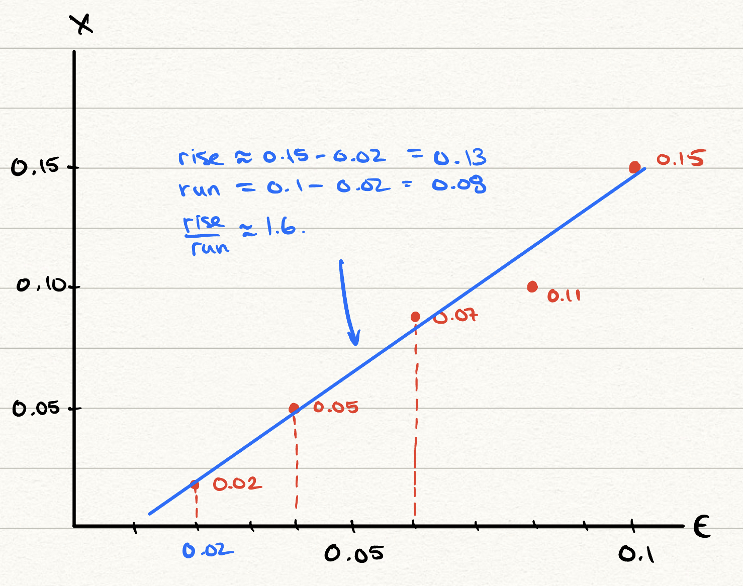
When doing this, I tried to fit to a line because I knew the error was supposed to be \[ x - x_0 \sim \epsilon \] so was expecting a line of unit gradient. But the gradient estimated above was a bit higher, at 1.6. Returning to Python, we see the problem.

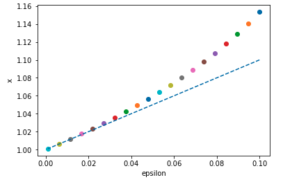
So over the range investigated of \(0.02 < \epsilon < 0.1\), the behaviour is quadratic.This is a nice lesson on how to discover new results based on computation and analysis.

By rescaling \(x\) appropriately in terms of \(\epsilon\), derive the first three terms of the asymptotic approximations of the remaining roots.

Solution

We expect the critical scaling to balance \(\epsilon x^3\) with \(x\) since these two will be dominant when \(x\) is large. So we set \[ x = \frac{X}{\sqrt{\epsilon}} \]

Now we have \[ X^3 - X + \sqrt{\epsilon} = 0. \]

You will notice that the progression here should go in powers of \(\epsilon^{1/2}\). Alternatively set \(\delta = \epsilon^{1/2}\) and now the problem is standard in \(\delta\): \[ X^3 - X + \delta = 0. \] And we expand \[ X = X_0 + \delta X_1 + \delta^2 X_2 + \ldots \] We get \[\begin{gather} X_0^3 - X_0 = 0 \Longrightarrow X_0^2 = 1 \Longrightarrow X_0 = \pm 1 \\ 3 X_0^2 X_1 - X_1 + 1 = 0 \Longrightarrow X_1 = -\frac{1}{2} \\ 3 X_0^2 X_2 + 3 X_0 X_1^2 - X_2 = 0 \Longrightarrow X_2 = \mp \frac{3}{8}. \end{gather}\] So it seems that the three-term approximation for the other two roots is \[ x \sim \frac{1}{\sqrt{\epsilon}} \left(\pm 1 - \sqrt{\epsilon} \frac{1}{2} \mp \epsilon \frac{3}{8}\right). \]

34.4 A damped projectile problem

If air resistance is included, then the non-dimensional toy model is instead \[\begin{gather} \frac{\mathrm{d}^2 y}{\mathrm{d}t^2} = - \frac{1}{(1 + \epsilon y)^2} - \frac{\alpha}{(1 + \epsilon y)} \frac{\mathrm{d}y}{\mathrm{d}t}, \\ y(0) = 0, \\ y'(0) = 1. \end{gather}\] where \(\alpha \geq 0\) is the parameter that controls air resistance.

Begin by assuming that \(\alpha\) is a fixed number and consider the limit where \(\epsilon \ll 1\). Find a one-term asymptotic expansion of the solution for small \(\epsilon\).

Solution

First, note that \[ (1 + \epsilon y)^{\alpha} = 1 + \alpha (\epsilon y) + O(\epsilon y)^2. \]

You will not need more terms than that. Substitute \(y = y_0(t) + \epsilon y_1(t) + \ldots\) into the equation. This gives, for the leading terms \[\begin{gather} y_0'' = -1 - \alpha y_0' \\ y_0(0) = 0 \\ y_0'(0) = 1 \end{gather}\] To solve this, you will need to refresh your memory on second-order differential equations learned in 2nd year. You can see Chapter 40 for references. To solve this set \(y_0 = e^{rt}\) and solve for \(r\) for the homogeneous equation. You will get \[ y_{\text{homogeneous}} = (c_1 + c_2 e^{-\alpha t}). \] From here, we need a particular solution. This can be obtained by guessing (also see this reference). If we guess \[ y_p = C t, \] we see that \[ y_p'' + \alpha y_p' = \alpha C = -1 \] implies \(C = -1/\alpha\). Therefore the general solution is \[ y_0 = (c_1 + c_2 e^{-\alpha t}) - \frac{t}{\alpha}. \] We now select the constants to satisfy the initial conditions. This yields \[ c_1 + c_2 = 0 \quad \text{and} \quad -\alpha c_2 - 1/\alpha = 1, \] from which the solution can be easily derived. It is \[ y(t) \sim \left(\frac{1}{\alpha^2} + \frac{1}{\alpha}\right) - \left(\frac{1}{\alpha^2} + \frac{1}{\alpha}\right)e^{-\alpha t} - \frac{t}{\alpha}. \]

The solution of \(y_1\) proceeds in the same way, but since we did not anticipate that this question would be so algebraically involved, we will not require solving for \(y_1\). This can be left as an exercise if you so wish.

(Challenging) Is the effect of the air resistance to increase or decrease the flight time? Justify based on your analytical solution.

Solution

The above solution seems quite strange. After all, when \(\alpha = 0\), we know that parabolic motion is expected. We found previously that \[ y_{\alpha = 0}(t) \sim -\frac{1}{2}t^2 + t. \] which matches our intuition about the expected flight being parabolic. However, notice that if \(\alpha\) is small, we can expand the exponential, \(e^{-\alpha t} = 1 - \alpha t + \ldots\). Substitution into the derived formula for \(y_0\) gives \[ \color{blue}y(t) \sim \left(\frac{1}{\alpha^2} + \frac{1}{\alpha}\right) - \left(\frac{1}{\alpha^2} + \frac{1}{\alpha}\right)\left[1 - \alpha t + \ldots\right] - \frac{t}{\alpha}. \] We can now simplify the expression and we see that the \(\alpha \to 0\) limit is not problematic, because it now becomes: \[ y_0 \sim \left(-\frac{1}{2}t^2 + t\right) + \alpha \frac{1}{6} \left(-3t^2 + t^3\right) + O(\alpha^2), \] and the previous terms that we believed might tend to infinity as \(\alpha \to 0\) cancel. Inspecting the above solution, notice that the leading-order result agrees with the previously derived result for \(\alpha = 0\). The next term shows the small effect of drag.

You can simply plot the curves and show the difference.

Figure 34.3: With (solid) and without damping (dashed)

Notice that the dashed line brings down the parabolic path initially.

34.5 ODE solvers and Euler’s method

Return to the setup of the above question.

Modify the script shown in Section 6.2 in order to solve the equation from the previous question at a prescribed value of \(\epsilon\) and \(\alpha\).

Solution

This is found in problemsets/sol02_solutions.ipynb.

Using a pocket calculator (or your phone calculator) apply Euler’s method with \(\Delta t = 0.2\), \(\epsilon = 0.2\), and \(\alpha = 1\) to determine the position of the projectile at \(t = 0.6\).

Solution

Euler’s method is simply \[ Y_{n+1} = Y_n + F(t_n, y_n)\Delta t. \] Here \[ F = \begin{pmatrix} y' \\ -\frac{1}{(1 + \epsilon y)^2} - \frac{\alpha}{(1 + \epsilon y)} \end{pmatrix}. \]

We split the time steps into {0, 0.2, 0.4, 0.6}. We also round to two figures.

t	Y	\(1 + \epsilon y\)	F	\(F \Delta t\)
0	(0, 1)	1	(1, -2)	(0.2, -0.4)
0.2	(0.2, 0.6)	1.04	(0.6, -1.5)	(0.12, -0.3)
0.4	(0.32, 0.3)	1.06	(0.3, -1.16)	(0.06, -0.23)
0.6	(0.38, 0.07)

After three iterations, we get a value of \(y(0.6) \approx 0.38\).

Compare your hand calculation with the result from the Python output, as well as with your asymptotic approximations.

Solution

We have (rounded to two digits) \[ \begin{aligned} y_{\text{exact numerical}} \approx 0.31 \\ y_{\text{euler}} \approx 0.38 \\ y_{\text{asym}} \approx 0.30 \end{aligned} \]