29 Problem set 4

Note

For feedback, hand in by Friday Week 6.

Q1. The wine cellar problem I

Within Chapter 12, the heat system was studied: \[ \begin{gathered} \frac{\partial T}{\partial t} = \kappa \frac{\partial^2 T}{\partial x^2}, \\ T(x = 0, t) = A \cos(\omega t), \\ |T(x, t)| \text{ is bounded as $x \to \infty$}. \end{gathered} \] for $x \geq 0$. The initial condition can be ignored.

The solution was sought in the form of $T(x, t) = G(t) H(x)$ using a separation of variables procedure leading to \[ \frac{G'}{G} = \kappa \frac{H''}{H} = \lambda. \] Go through an argument that the cases of $\lambda = 0$ and $\lambda$ real lead to incompatible solutions. Review the calculation that $\lambda = i\omega$ leads to the desired solution given in (Equation 12.1).

Q2. The wine cellar problem II

Review the code written in lecture15-winecellar.ipynb.

Verify how well the numerical solution matches the exact analytical solution by overlaying the numerical solution with the analytical solution.

Investigate the solutions under different choices of parameters and time-stepping tolerances until you are confident you know how the numerical algorithm works.

Q3. EBMs with variable sun

Satellite data indicates that $Q$, varies roughly between 341.37 W/m² and 341.75 W/m², with a period of about 11 years.

Use the simple EBM given in (Equation 13.3) and repeated below: \[ Q(1 - a) = \sigma \gamma T^4, \] with a constant albedo, $a = 0.3$ and greenhouse gas factor $\gamma = 0.6$ to estimate the resultant variation (max and min) in the Earth’s mean surface temperature $T$.
Similar to (a) but this time, use the Budyko balance equation, \[ Q(1 - a) = A + BT \] with $A = 203.3 \, \mathrm{W} \mathrm{m}^{-2}$ and $B = 2.09 \, \mathrm{W}/(\mathrm{m}^{2} \, {}^\circ \mathrm{C})$ to estimate the resultant variation in the surface temperature. Use $a = 0.3$.
The actual variation in surface temperature is in fact less than what you computed above. Why might this be?

Q4. EBMs and phase line analysis

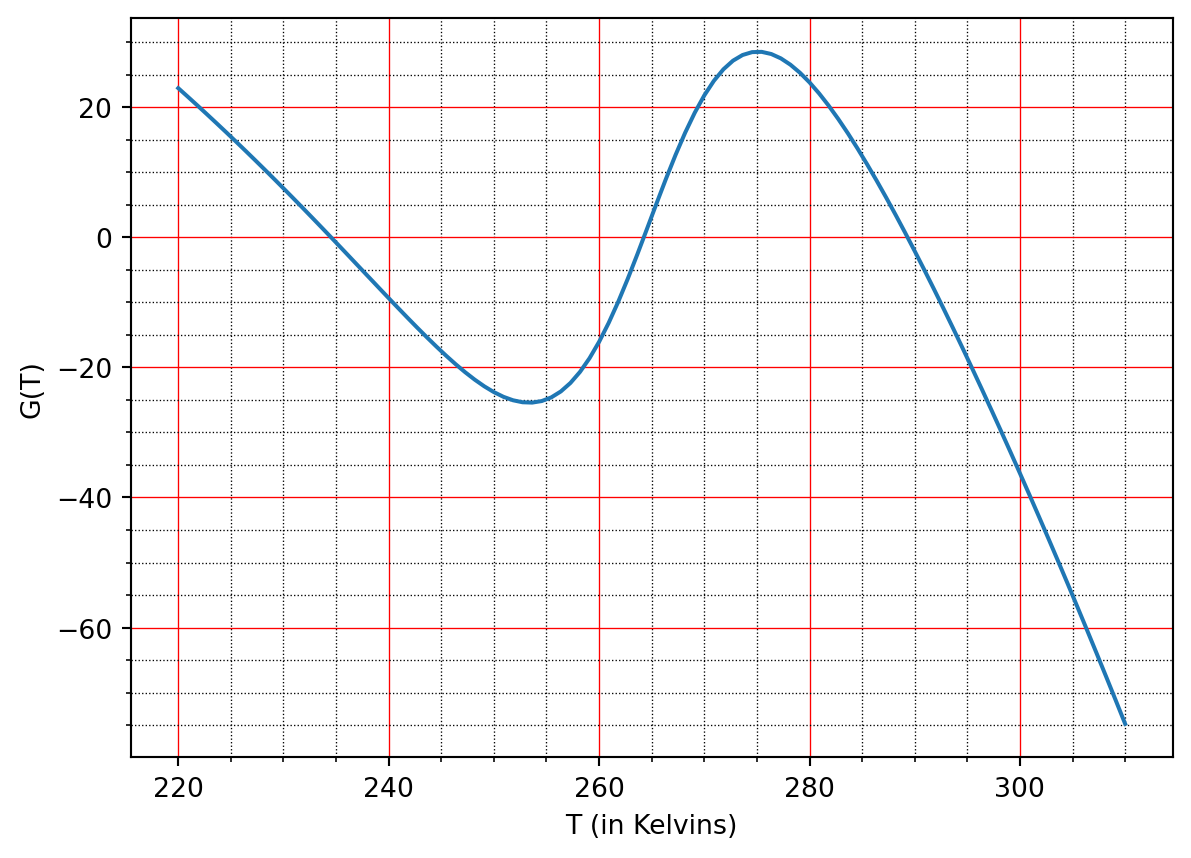
Consider the energy balance equation \[ C \frac{\mathrm{d}T}{\mathrm{d}t} = Q(1 - a(T)) - \sigma \gamma T^4 \equiv G(T). \tag{29.1}\] with $a$ given by (Equation 13.2). Because the differential equation is autonomous, we can apply phase-line analysis in order to qualitatively understand the evolution. Below is a plot of the function $G$:

import numpy as np
import matplotlib.pyplot as plt

Q = 342; sigma = 5.67e-8; gam = 0.6;
a = lambda T: 0.5 - 0.2*np.tanh(0.1*(T-265));
T = np.linspace(220, 310, 100);
G = Q*(1-a(T)) - sigma*gam*T**4
fig, ax = plt.subplots()
ax.plot(T, G)
ax.grid(); ax.minorticks_on();
# Customize the major grid
ax.grid(which='major', linestyle='-', linewidth='0.5', color='red')
# Customize the minor grid
ax.grid(which='minor', linestyle=':', linewidth='0.5', color='black')
plt.xlabel('T (in Kelvins)'); plt.ylabel('G(T)');

Sketch the solution $T(t)$ of this equation for $t > 0$ if $T(0) = 230, 240, 260, 270$ and $300$.
Sketch the solution $T(t)$ of this equation for $t > 0$ if $T(0) = 285$. Then sketch the solution of this equation with the same initial data in the same coordinate system if $C$ is twice as large. Explain your answer.
If $\gamma$ is decreased due to the increased greenhouse effect, the entire curve is shifted upwards. Sketch the solution if $T(0) = 280$. Sketch the solution with the same initial data if $\gamma$ is decreased. Explain your answer.