24 Problem set 1
The intention of this problem set is to practice concepts from material related to conservation laws and non-dimensionalisation. Although these concepts seem quite separate from “Maths of Planet Earth”, actually, they form important pillars of mathematical modelling.
Q1. Bump lemma
Prove the following one-dimensional lemma, which was used in the derivation of the heat equation.
If \(\int_a^b g(x) \, \mathrm{d}x = 0\) for all \(a\) and \(b \in [0, 1]\), then \(g(x) \equiv 0\) for all \(x\in [0, 1]\).
Hint: think of a proof by contradiction.
Q2. A source in the heat equation
Consider the same heat experiment discused in Chapter 2 but now consider a bar that has an internal source or sink generating or removing heat, such as the case of a boiler with an internal heating element. By adapting a similar derivation to the one presented, explain why the modified conservation of heat equation is \[ \frac{\mathrm{\partial}}{\mathrm{\partial}t} \int_a^b \rho c T \, \mathrm{d}x = q(x = a, t) - q(x = b, t) + \int_a^b R(x, t) \, \mathrm{d}x. \]
In addition:
By studying the dimensions of the other terms in the above equation, find what the dimensions of \(R\) are. What does \(R > 0\) mean and \(R < 0\)?
Hence derive the partial differential equation that governs the temperature \(T\).
By introducing the appropriate scalings on each of the variables, \(x\), \(t\), and \(T\), non-dimensionalise the PDE and discuss the non-dimensional parameters (there will be two).
Q3. The unique timescale in the heat equation
During our investigation of the heat equation, we found that it was possible to scale time so as to scale out the only non-dimensional parameter that appears in the PDE (\(\Pi\)). This produced (Equation 3.1). The disappearance of all non-dimensional parameters is due to the fact that only a single sensible timescale exists.
By adjusting the boundary conditions, we may create a new problem involving heat flow where a unique ‘special’ timescale can no longer be chosen.
Consider a system where one side of the rod is heated in some periodic fashion, e.g. set the initial and boundary conditions to be \[ \begin{aligned} T(x, 0) &= T_0 \\ T(0, t) &= T_a \cos (\omega t), \\ T(L, t) &= T_b. \end{aligned} \]
What must the units of \(\omega\) be?
Non-dimensionalise as usual and, without selecting the timescale, \([t]\), identify the key non-dimensional parameters that remain. Write a brief sentence to describe their physical interpretation.
There are two sensible choices for setting the timescale, \([t]\). Identify the two choices and present the reduced set of equations in each case.
Q4. Timescale in the surface energy
Take the basic zero-dimensional energy model studied in (Equation 4.7) for the temperature of the troposphere: \[ C \frac{\mathrm{d}T}{\mathrm{d}t} = \frac{1}{4} Q(1 - a) - \sigma \gamma T^4. \]
Non-dimensionalise the model by choosing \(T = [T]T'\), \(t = [t]t'\), and \(Q = [Q]Q'\). Show that it is possible to select the scalings on the temperature and time so as to completely remove all constants from the problem when \(Q\) is assumed to be constant.
Thus, show that the analysis of the above equation is equivalent to studying \[ \frac{\mathrm{d}T}{\mathrm{d}t} = 1 - T^4, \] where we have dropped the primes and assumed that the albedo is such that \(1 - a \neq 0\).
From your choice of \([t]\), estimate the typical dimensional value using \(d \approx 10 \mathrm{km}\), \(\rho \approx 1 \mathrm{kg} \,\mathrm{m}^{-3}\), \(c_p \approx 10^3 \mathrm{J} \,\mathrm{kg}^{-1} \,\mathrm{K}^{-1}\).
Use a pocket calculator to verify your calculations and conclude that this time-scale is on the order of a month. What is the relevance of this approximation as it concerns the steady-state solution?
Q5. Choice of scalings in Navier Stokes
Suppose that the time, with \(t = [t]t'\) is non-dimensionalised as \([t]=\frac{1}{f}\) where \(f\) is a frequency. Show that the Navier-Stokes equations, introduced in Problem Class 2, can be written as \[
\frac{\partial \boldsymbol{u}}{\partial t}+\frac{1}{\text{St}}\left( \boldsymbol{u} \cdot \nabla \right)\boldsymbol{u}=-\nabla p+\frac{1}{\text{Re}} \nabla^2 \boldsymbol{u}.
\] Above, the Reynolds number is defined via \(\text{Re} = \frac{f L^2}{\nu}\) and the Strouhal number is defined via \(\text{St} = \frac{L f}{U}\). The Strouhal number represents the effect of vortex shedding in flow across an object. The higher \(\text{St}\) is, the more vortices will be generated by the flow. 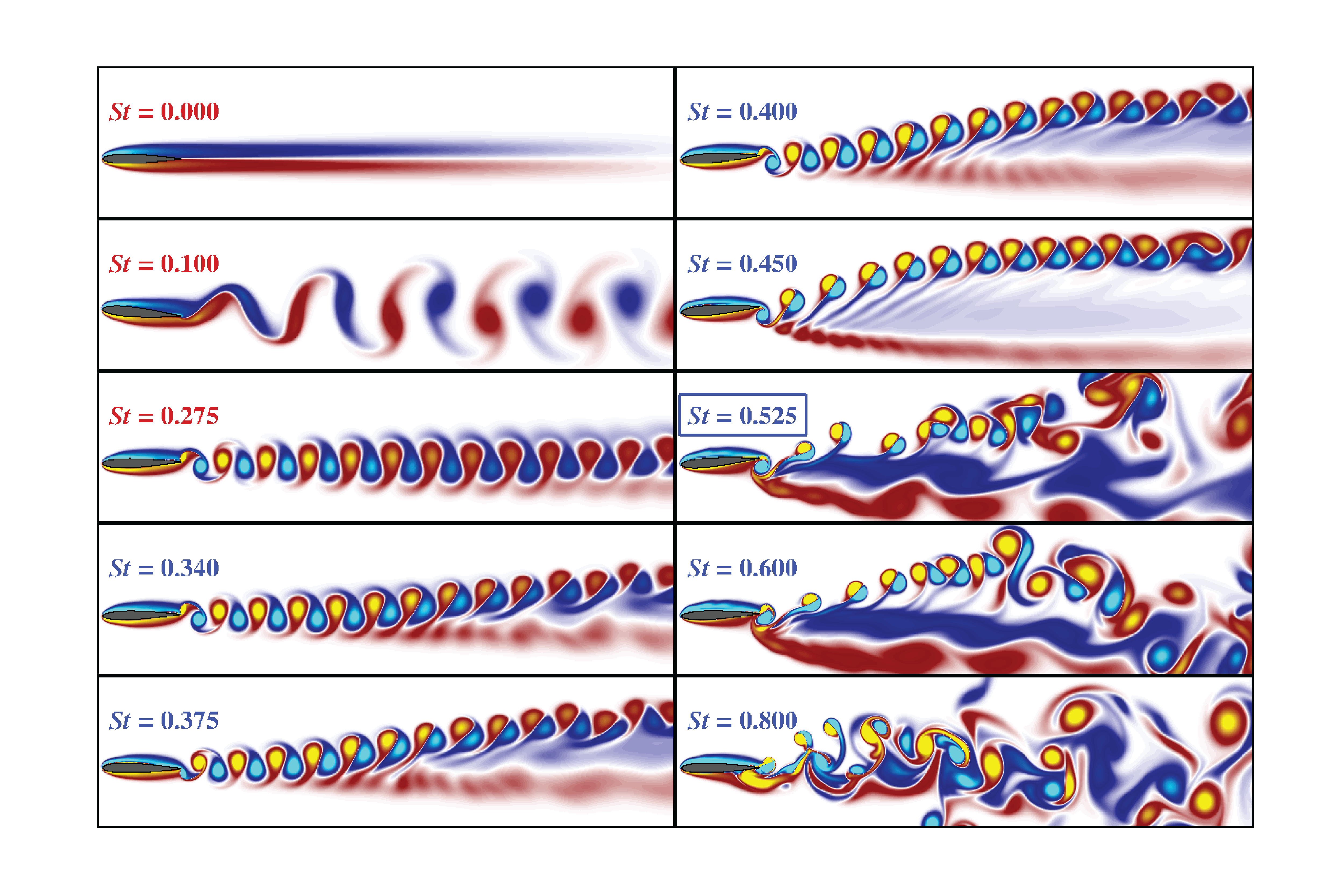
By considering the SI units for the different quantities of \(f\), \(L\), \(\nu\), and \(U\), confirm that the two non-dimensional numbers introduced above are indeed non-dimensional.