One powerful set of techniques for approximating solutions to equations is called asymptotic analysis or perturbation theory. To begin with, in this chapter, we introduce you to these techniques as a means to approximating the solutions to equations like: \[
\epsilon x^2 + x - 1 = 0,
\] when \(\epsilon\) is a small parameter.
Soon, we apply the techniques to approximating solutions of differential equations.
5.1 A simple quadratic
A singular quadratic
Consider the solution of \[
\epsilon x^2 + x - 1 = 0,
\tag{5.1}\] where \(\epsilon\) is a fixed and very small positive number, say \(0.000001\). Forget that we know how to solve a quadratic equation: is it possible to develop a systematic approximation method?
If \(\epsilon = 0\), then \(x = 1\). Moreover, if we substitute \(x = 1\) into the equation, then we see that the error is small and proportional to \(\epsilon\). It is natural to seek an approximation in powers of \(\epsilon\). We call this an . We write \[
x = x_0 + \epsilon x_1 + \epsilon^2 x_2 + \ldots
\] Substitution into the equation yields \[
\epsilon \Bigl(x_0 + \epsilon x_1 + \epsilon^2 x_2 + \ldots\Bigr)^2 + \Bigl( x_0 + \epsilon x_1 + \epsilon^2 x_2 + \ldots \Bigr) - 1 = 0.
\] Expand and collect terms in powers of \(\epsilon\): \[
\Bigl( x_0 - 1 \Bigr) + \epsilon\Bigl(x_1 + x_0^2\Bigr) + \epsilon^2\Bigl(x_2 + 2 x_0 x_1\Bigr) + \ldots = 0.
\] Now we equate coefficients at each order in \(\epsilon\). This gives \[
\begin{aligned}
x_0 - 1 &= 0 \Longrightarrow x_0 = 1 \\
x_1 + x_0^2 &= 0 \Longrightarrow x_1 = -1 \\
x_2 + 2 x_0 x_1 &= 0 \Longrightarrow x_2 = 2
\end{aligned}
\] We therefore have obtained the three-term approximation, \[
x = 1 - \epsilon + 2\epsilon^2 + \ldots
\] Clearly we could continue this process ad infinitum obtaining increasingly accurate approximations to one of the roots.
5.1.1 The singular root
\(\nextSection\)
But where has the other quadratic root gone?
The problem is that in considering \(\epsilon\) to be small, we began by ignoring the leading term, \(\epsilon x^2\). We effectively assumed that the equation was primarily balanced by setting the \(x\) term with the \(-1\) term, and the sum of the two terms approximately equalling zero.
But if \(|x|\) is large, then clearly our assumption that \(\epsilon x^2\) being small may not be necessarily true for it depends on how large \(|x|\) is compared to \(\epsilon\). Note that if \(|x|\) is large, then necessarily the last term, \(-1\), is negligible in comparison. Therefore, in order for \(\epsilon x^2\) to balance \(x\), we see that \(|x|\) must be of size \(1/\epsilon\).
Therefore this suggests that we should re-scale our solution as follows \[
x = \frac{X}{\epsilon}.
\]
Substitution into the original quadratic now yields \[
X^2 + X - \epsilon = 0.
\] Now notice that \(\epsilon = 0\) expresses the correct balance in order to detect that missing root. Again we write \[
X = X_0 + \epsilon X_1 + \epsilon^2 X_2 + \ldots
\] and attempt to solve order by order. Substitution into the equation yields \[
\Bigl(X_0 + \epsilon X_1 + \epsilon^2 X_2 + \ldots\Bigr)^2 + \Bigl(X_0 + \epsilon X_1 + \epsilon^2 X_2 + \ldots\Bigr) - \epsilon = 0.
\] Expand and collect orders of \(\epsilon\): \[
\begin{aligned}
X_0^2 + X_0 &= 0 \Longrightarrow X_0 = -1 \\
2X_0 X_1 + X_1 -1 &= 0 \Longrightarrow X_0 = -1,
\end{aligned}
\] and thus to two orders, we have \[
X = -1 - \epsilon + \ldots \Longrightarrow x = - \frac{1}{\epsilon} - 1 + \ldots
\]
Of course, we have used a very simple example (a solvable quadratic) to illustrate the idea of asymptotic approximations, but you should hopefully see that this method is extensible to much more complicated equations.
5.2 Order notation and the tilde sign for asymptotic
\(\nextSection\)
We define precisely what we mean when we say that two functions, say \(f\) and \(g\), exhibit the same behaviour in some limit, say \(\epsilon \to 0\) or \(x \to x_0\) or \(x \to \infty\) and so forth. For instance, we claim that the graphs of \(\sin(x)\) and \(x\) look very similar as \(x \to 0\). Thus we might write \[
\sin(x) \sim x \quad \text{as $x \to 0$.}
\tag{5.2}\]
This notation of similarity allows us to specify functional behaviours at a deeper level than just limits. As you can see, it is not as useful to specify that \[
\lim_{x \to 0} \sin{x} = \lim_{x\to 0} x.
\] In contrast, the asymptotic relation is much more prescriptive about the way that the functions are approaching the limit.
Definition of \(\sim\), \(\gg\), and \(\ll\)
First, the notation \[
f(x) \ll g(x), \qquad x \to x_0,
\] is read as “\(f(x)\) is much smaller than \(g(x)\) as \(x \to x_0\)” and means \[
\lim_{x\to x_0} \frac{f(x)}{g(x)} = 0.
\] We may analogously use \(g(x) \gg f(x)\) for “much greater than”.
Second, the notation \[
f(x) \sim g(x), \qquad x \to x_0,
\] is read as “\(f(x)\) is asymptotic to \(g(x)\) as \(x \to x_0\)”, and means that the error between \(f\) and \(g\) tends to zero as \(x \to x_0\), or \[
\lim_{x\to x_0} \frac{f(x)}{g(x)} = 1.
\] We will often say “\(f\) is like \(g\)” or “\(f\) behaves like \(g\)”,
Here are some examples.
Examples
\(\sin x \sim x \sim \tan x\) as \(x \to 0\)
\(x^2 + x + 1 \sim \dfrac{x^3 + \sin x}{1 + x}\) as \(x \to \infty\)
\(\sin x \ll \cos x\) as \(x \to 0\)
In the examination of limiting processes, often the main issue of consideration is the relative sizes of quantities defined according to their powers. For example, if \(x\) is a very small number, with \(x = 10^{-5}\), then \(x^5\) is much smaller than \(x\) (in terms of our notation, \(x^5 \ll x\) as \(x \to 0\)). On the other hand, we might not care so much about the difference between \[
x^5 \quad \text{vs.} \quad 5 x^5
\] The point is that the of \(x^5\) and \(5 x^5\) is the same as \(x \to 0\). The “Big-Oh” notation formalises this distinction.
Definition of Big-Oh
We write \(f = O(g)\) as \(x \to x_0\) to mean that there exists constants \(K > 0\) and \(x^* > 0\) such that \[
|f| < K |g| \quad \text{for all $|x - x_0| < x^*$}.
\]
In practice, the use of the order symbol is very natural and you will not need to work with the technical definition. For example, when you derive the terms of the Maclaurin/Taylor series, you are naturally clustering all the terms of the same order (power) together. For us, the \(O\) symbol provides a very convenient way of separating terms of different sizes.
Examples
\(2\sin x = O(\tan x)\) as \(x \to 0\)
\(x^2 + x + 1 = O\left(\dfrac{5x^3 + \sin x}{1 + x}\right)\) as \(x \to \infty\)
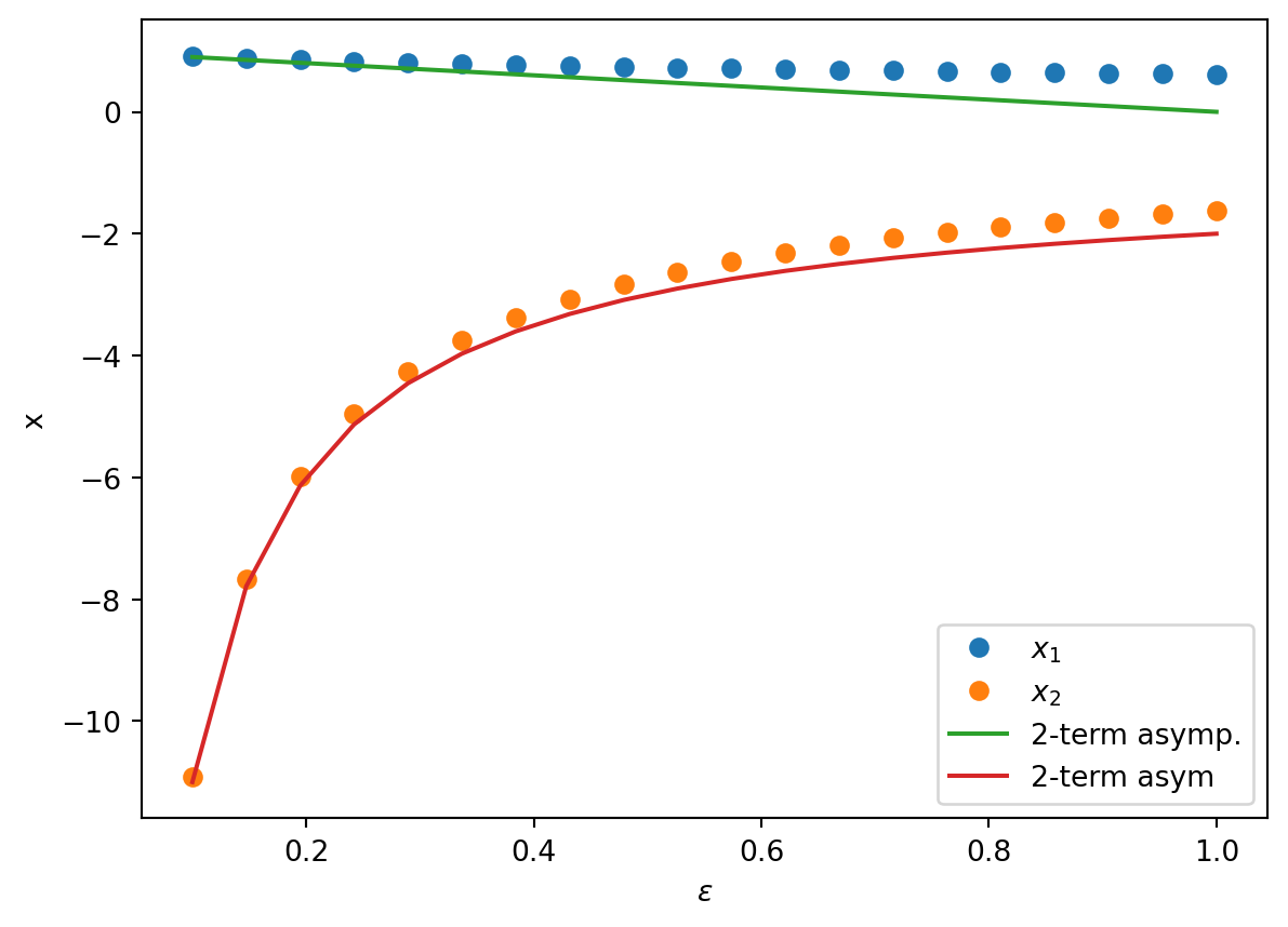
Let us return to the case of the quadratic example (Equation 5.1). Using the O notation, we can write \[
x =
\begin{cases}
1 - \epsilon + 2 \epsilon^2 + O(\epsilon^3) \\
-\frac{1}{\epsilon} - 1 + O(\epsilon^2)
\end{cases}
\] for the two roots. Alternatively, we can truncate the expansions and simply using the \(\sim\) symbol: \[
x \sim
\begin{cases}
1 - \epsilon \\
-\frac{1}{\epsilon} - 1
\end{cases}
\]