35 Problem set 5 solutions
Q1. Evolution
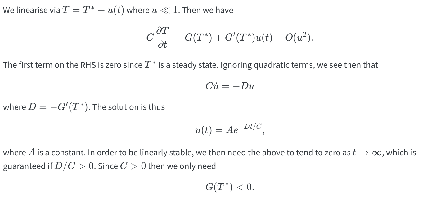
Consider again the basic time-dependent EBM given in (Equation 27.1). Let \(T^*\) be a steady-state solution and set \(T = T^* + u(t)\) where \(u(t)\) is a small perturbation from the steady state.
- Show that the perturbation satisfies \[ C \dot{u} = -D u + O(u^2). \] and hence solve for the general solution of the leading-order perturbation (ignoring quadratic terms). What are the conditions on \(T^*\) so that the steady state is linearly stable?
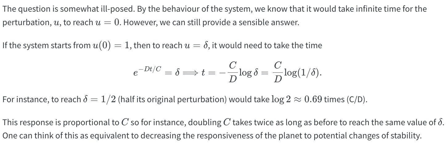
- Assuming \(T^*\) is linearly stable, find the typical response time to a perturbation. For instance, what is the time it takes for the perturbation to reach the value \(u(t) = 0\) if \(u(0) = 1\)? How does this response time change with \(C\)? What is the physical interpretation of this regarding the climate?
Q2. Integral of energy over the planet
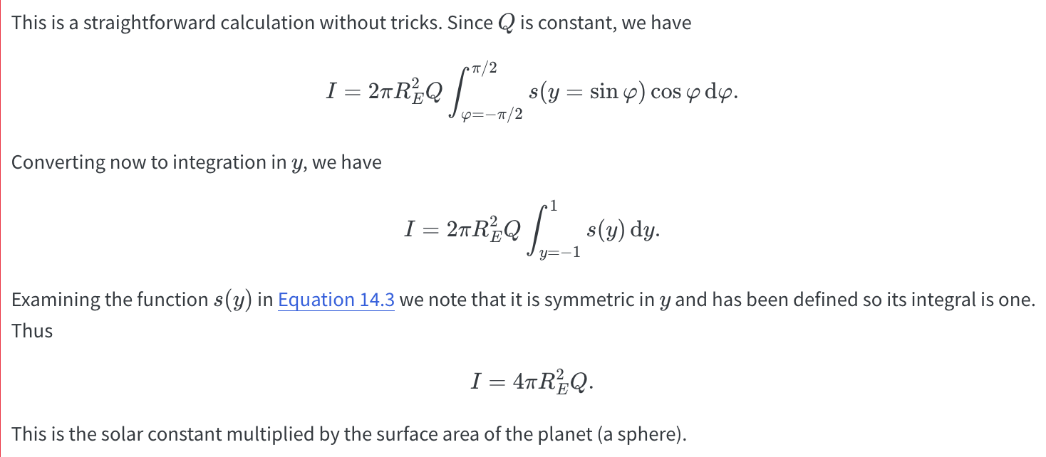
Ignoring the effects of albedo, the total radiation absorbed over the surface of the planet (per unit time) is given by \[ \iint_{\text{planet}} Qs(y=\sin\varphi) \, \mathrm{d}S. \] This is what is known as a surface integral (Section 46.1). In the case of the spherical coordinate system, this is calculated by \[ \int_{\theta=0}^{2\pi} \int_{\varphi = -\pi/2}^{\pi/2} Qs(y = \sin\varphi) R_E^2 \cos\varphi \, \mathrm{d}\varphi \mathrm{d}\theta. \] Use the properties of \(s(y)\) in (Equation 13.3) to conclude that the total radiation absorbed is \(4\pi R_E^2 Q\).
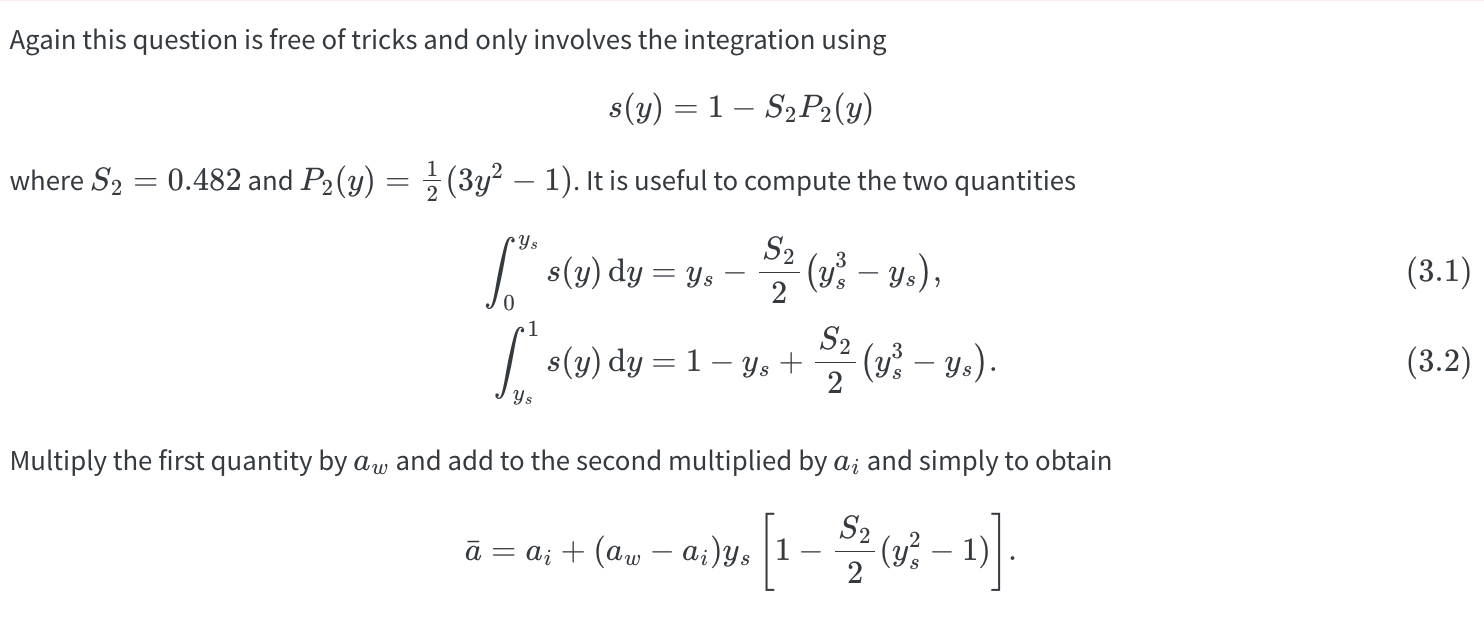
Q3. Mean temperature in the latitude-dependent EBM
Consider now the latitude-dependent EBM \[ C \frac{\mathrm{\partial}T}{\mathrm{\partial}t} = Qs(y)[1 - a(y)] - (A + BT) + k(\bar{T} - T). \] Recall the albedo is given by \(a = a_i\) for \(y > y_s\) and \(a = a_w\) for \(y < y_s\).
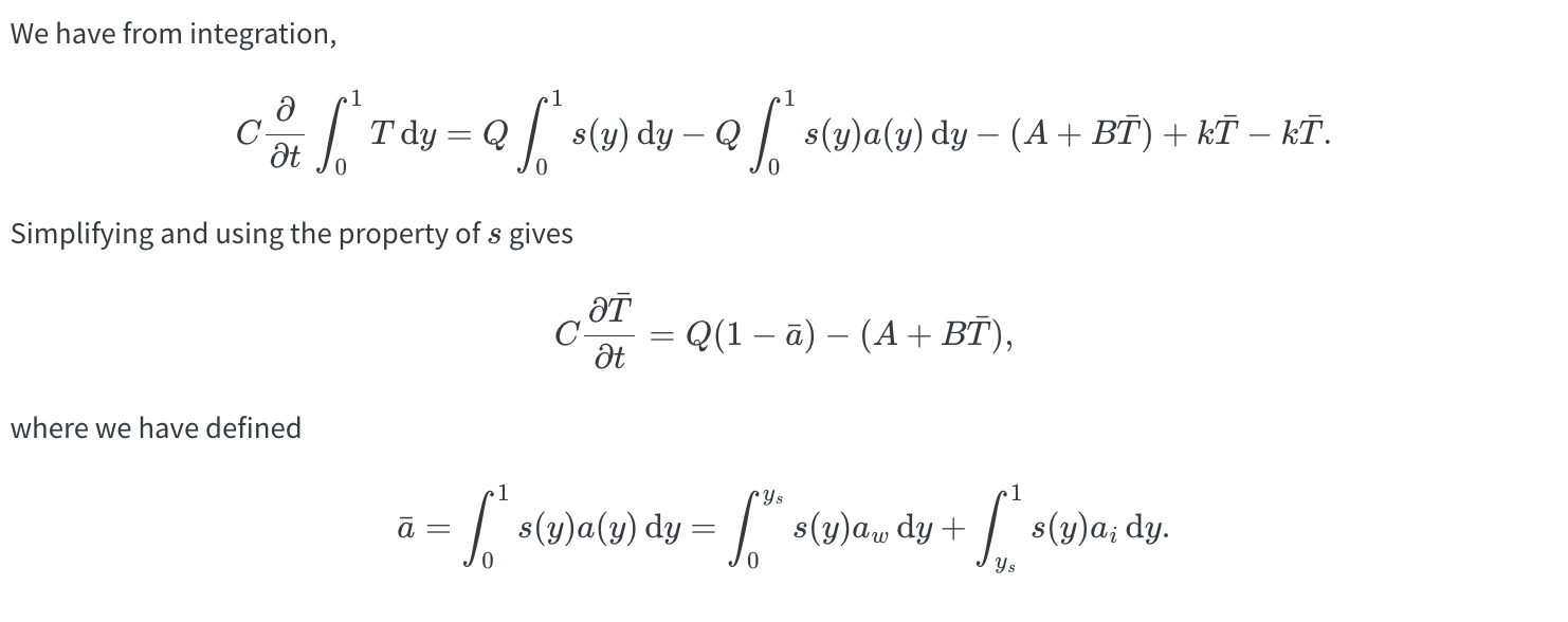
- By integrating the above equation over \(y \in [0, 1]\), show that the mean temperature is given by \[ C \frac{\mathrm{d}\bar{T}}{\mathrm{d}t} = Q(1 - \bar{a}) - (A + B\bar{T}), \tag{35.1}\] where \[ \bar{a} = \int_0^1 s(y) a(y) \, \mathrm{d}y = \alpha_w \int_0^{y_s} s(y) \, \mathrm{d}y + a_i \int_{y_s}^1 s(y) \, \mathrm{d}y. \]
- In the case that \(s\) is given by (Equation 13.3), show that \[ \bar{a} = a_i + (a_w - a_i) y_s[1 - 0.241(y_s^2 - 1)]. \tag{35.2}\] What is \(\bar{a}\) in the two situations of a completely ice-covered world and an ice-free world?
Q4. Sensitivity of the climate
Consider the equation for the global average temperature given in (Equation 35.1): \[ C \frac{\mathrm{d}\bar{T}}{\mathrm{d}t} = Q(1 - \bar{a}) - (A + B\bar{T}). \] We would like to understand how the climate behaves under a small perturbation in the solar forcing. In general, though, the ‘constants’, \(A\), \(B\), and \(\bar{a}\) will depend on \(T\). For example, their values may have been calibrated under a static situation. Therefore, let \(A = A(T)\), \(B = B(T)\), and \(\bar{a} = \bar{a}(T)\).
Below, we drop all bars for convenience.
- Consider a perturbation of the solar radiation, say \(Q = Q_0 + \delta\) where \(\delta\) is small in comparison to \(Q_0\). Expand now the temperature into a series: \[ T = T_0 + \delta T_1 + \ldots \] Show that at \(O(\delta)\), the perturbation is governed by \[ C \frac{\mathrm{d}T_1}{\mathrm{d}t} = (1 - a(T_0)) - B(T_0) T_1 - A'(T_0) T_1 - T_0 B'(T_0) T_1 - Q_0 a'(T_0) T_1. \]
- Consequently, show that the temperature perturbation can be written as \[ B(T_0) \tau \frac{\mathrm{\partial}T_1}{\mathrm{\partial}t} = [1 - a(T_0)] - \frac{B(T_0)}{g} T_1, \tag{35.3}\] where
\[ \begin{aligned} \tau &= \frac{C}{B(T_0)} \\ g &= \frac{1}{1-f} \\ f &= f_1 + f_2 \\ f_1 &= \frac{1}{B(T_0)} \left(-T_0 B'(T_0) - A'(T_0)\right),\\ f_2 &= \frac{1}{B(T_0)} \left(-Q_0 a'(T_0)\right) \end{aligned} \]
The parameter \(\tau\) measures the time scale of the climate system’s thermal inertia. It involves the thermal inertia of the atmosphere and also the much larger inertia of the oceans. The factor \(g\) is the climate gain; it amplifies any response to the radiative perturbation by a factor of \(g\). Also \(f_1\) incorporates the effect of water-vapor feedback and \(f_2\) that of ice and snow albedo feedback.
- Consider (Equation 35.3) at steady state, so therefore the perturbed equilibrium temperature is equal to \[ \delta T_1 = \frac{[1 - a(T_0)] \delta g}{B(T_0)}. \] If the CO2 level in the atmosphere doubles, then the radiative forcing might be adjusted as: \[ (1 - a(T_0)) \delta = 3.7 \, \mathrm{W} \cdot \mathrm{m}^{-2}. \] Assuming that the climate gain is \(g = 3\) and \(B(T_0) = 1.9 \mathrm{W} \cdot \mathrm{m}^{-2} \cdot ({}^\circ \mathrm{C})^{-1}\), what is the expected increase in temperature?