Q1. Non-dimensionalisation of the Stommel box model
Consider the Stommel box model given in (Equation 22.1). Non-dimensionalise the model in order to produce the set of equations given in (Equation 22.2), repeated here: \[
\begin{aligned}
\frac{\mathrm{d}x}{\mathrm{d}t} &= \delta(1 - x) - |f(x, y)|x, \\
\frac{\mathrm{d}y}{\mathrm{d}t} &= 1 - y - |f(x, y)|y,
\end{aligned}
\] where we have introduced the function, \[
f(x, y; R, \lambda) = \frac{1}{\lambda}(Rx - y),
\]
Provide a brief description of the physical interpretations of the parameters \(\lambda\), \(\delta\), and \(R\).
The non-dimensionalisation procedure was done in the lecture notes and lectures.
The final parameters were established by \[
\delta = \frac{d}{c}, \qquad \lambda = \frac{c}{2\alpha k \Delta T^*}, \qquad R = \frac{\beta \Delta S^*}{\alpha \Delta T^*}.
\] Their interpretations are as follows: \(\delta\) measures the relative relaxation temporal rates of the salt-basin exchange and the temperature-basin exchange. Since thermal energy turns out to exchange on a faster time scale than salinity, then we are typically interested in \(\delta \ll 1\).
The parameter \(\lambda\) is a measure of the strength of the THC. For example, with \(k\) large, this corresponds to significant flow through the pipes connecting the boxes, and so \(\lambda \to 0\) corresponds to strong THC.
Finally \(R\) allows us to compare the relative effects of temperature and salinity differences between the external basins. Salinity differences dominate if \(R > 1\) and temperature differences dominate if \(R < 1\).
Q2. Investigations for \(R\)
\(\nextSection\)
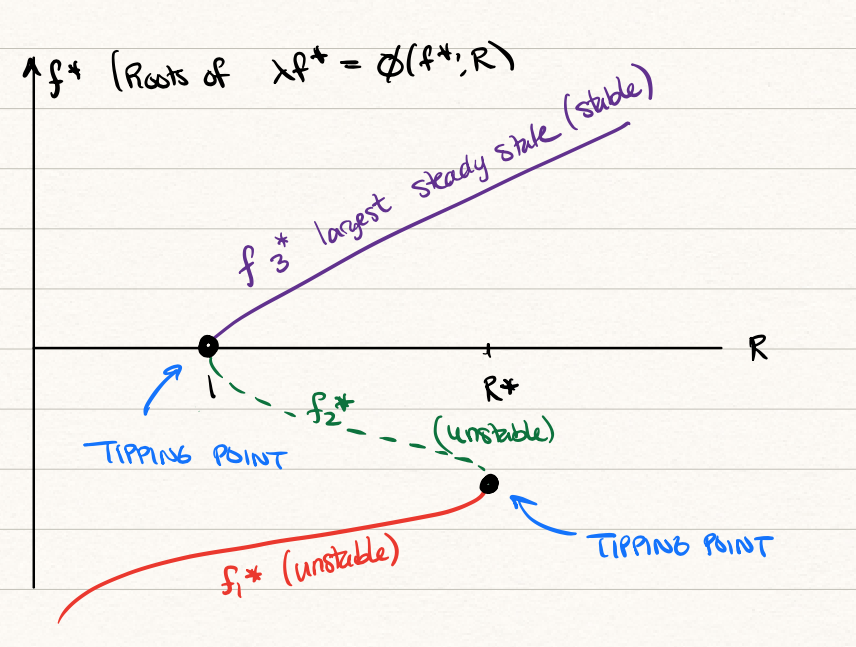
Using the script available on Noteable investigate the behaviour of the Stommel box model under changing values of \(R\) and fixed values of the other parameters. Based on your intuition, what do you expect to be the features of the bifurcation diagram, as shown in the \((R, f)\)-plane?
Remember that the steady states are found by examining the intersections of the curves \(\lambda f = \phi\). From (Equation 22.5), we have \[
\phi(f^*) = \frac{\delta R}{\delta + |f^*|} - \frac{1}{1 + |f^*|}.
\] so essentially the effect of changing \(R\) is to multiply the curve \(\phi\) by a multiplier. Using the code on the JupyterHub we obtain the following graph for different values of \(R\).
For the smallest values of \(R\), note that only the lowermost steady state will be present. As \(R\) crosses the critical value of \(R = 1\), two intersections are borne at \(\phi = 0\). Eventually \(R\) crosses another critical value, and the two leftmost intersections merge then disappear, leaving only the largest steady-state.
Because the stability of the solution is essentially given by the ordering of the curves (if the curve \(\lambda f\) is larger than the curve \(\phi\) on the left of the steady-states), then we can see that, as typical for stability in this course, the first and third steady states are stable, and the middle one unstable.
We can now plot a bifurcation diagram using the above information.
Q3. Alternative scalings of the Stommel box model
\(\nextSection\)
It is possible to scale the problem differently, and this may allow for simpler analysis. Consider the set of equations in Q1. Write instead \[
x = [x] s, \qquad y = [y] \theta, \qquad t = [t] t',
\] Choose the correct scalings, \([x]\), \([y]\), and \([t]\), so that we obtain a re-scaled version: \[
\begin{aligned}
\frac{\mathrm{d}s}{\mathrm{d}t'} &= 1 - (\epsilon + |q|) s, \\
\frac{\mathrm{d}\theta}{\mathrm{d}t'} &= 1 - (\mu + |q|)\theta,
\end{aligned}
\]
where now the flow term is given by \[
q = \kappa(-\theta + \tilde{R}s).
\] In addition to the choice of scalings, you will need to describe how the new parameters, \(\epsilon\), \(\mu\), \(\kappa\), and \(\tilde{R}\), are related to the older parameters.
Putting in the scalings, \[
\begin{aligned}
\frac{[x]}{[t]}\frac{\mathrm{d}s}{\mathrm{d}t'} &= \delta(1 - [x]s) - [x]|f(x, y)|s, \\
\frac{[y]}{[t]}\frac{\mathrm{d}\theta}{\mathrm{d}t'} &= 1 - [y]\theta - |f(x, y)|\theta.
\end{aligned}
\]
Comparing the equations, we see that we should choose \[
[x] = \epsilon, \qquad \frac{\delta [t]}{[x]} = 1, \qquad [t] = \mu, \qquad [y] = [t] = \mu.
\] Under this choice, \[
\begin{aligned}
\frac{\mathrm{d}s}{\mathrm{d}t'} &= 1 - \epsilon s - [t]|f(x, y)|s, \\
\frac{\mathrm{d}\theta}{\mathrm{d}t'} &= 1 - \mu\theta - [t]|f(x, y)|\theta.
\end{aligned}
\] The latter quantity is \[
\mu f = \frac{\mu[y]}{\lambda}\left(-\theta + \frac{R[x]}{[y]}s\right).
\] We there write \[
\kappa = \frac{\mu[y]}{\lambda}, \qquad \tilde{R} = \frac{R[x]}{[y]}
\]
Thus we have produced \[\begin{align}
\frac{\mathrm{d}s}{\mathrm{d}t'} &= 1 - \epsilon s - |q|s, \\
\frac{\mathrm{d}\theta}{\mathrm{d}t'} &= 1 - \mu\theta - |q|\theta.
\end{align}\] where \[
q = \kappa(-\theta + \tilde{R}s).
\]
Q4. Box models for flooding 1
\(\nextSection\)
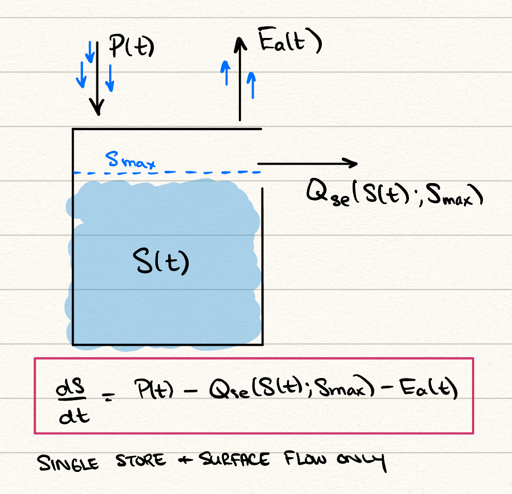
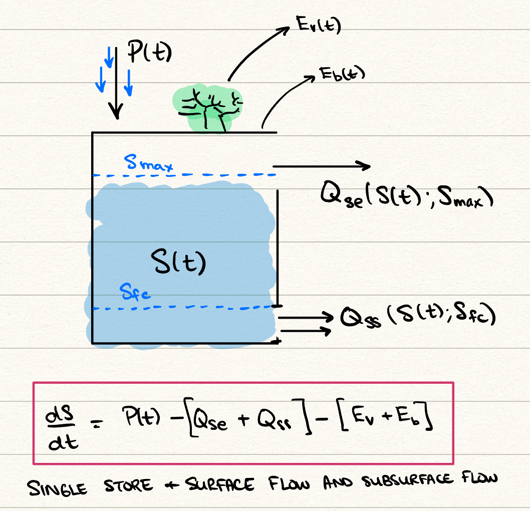
- In Chapter 23, two models for flooding were proposed. These models are conceptual models (or so-called box models), like the ones used previously in our study of the ocean. Create a diagram of the two box models, using arrows to indicate inputs and outputs. Label annotations related to precipitation, evapotranspiration, and runoff.
A box diagram of the model where only a surface flow is modelled with a threshold \(S_m\) is given as:
A box diagram of the model where both a surface and subsurface flow is modelled is given as:
The second model also has additional evapotranspiration modelled for vegetative cover and bare soil.
- The analysis of the flood models contains numerous interesting complexities that seem very different than what you may have observed in your undergraduate courses on dynamical systems and differential equations (it is a shame this comes nearly at the last possible week in your studies!). Examining the form of the associated differential equations, name several reasons why the analysis of such equations is difficult and beyond what you may have studied in Year 2 differential equations (and beyond).
Here are a few possible complexities:
- The flood models may seem linear, but in fact the presence of the switching functions, \(\sigma(S - S_0) = H(S - S_0)\) (the step functions or similar) are functions of \(S\) themselves. Therefore, the equations are nonlinear. Conventional techniques are not immediately applicable.
- The function like the precipitation, \(P(t)\), is unspecified and typically found by data analysis. It is not clear that this function is smooth and well-defined (and in fact, we typically think of it as stochastic). It is not obvious that we can attempt to perform analysis making simplified assumptions on \(P(t)\) (say that it is constant or sinusoidal).
- If \(P\) is non-smooth, what does this mean about numerical computation? Are we justified in using typical numerical techniques (like Euler’s method)?
- The differential equations are accompanied by potentially many parameters. It is not immediately clear how complicated the space of solutions is; is the calibration of such parameters even a well-posed endeavour?
- The equations are non-autonomous. So your conventional analysis by phase planes or phase lines is immediately more difficult.
It is good to end the course on such an example, and in order to appreciate that despite the fact you have learned much mathematics and differential equations theory, even apparently simple models conventionally used by hydrologists are, on the surface, `beyond’ your traditional analysis.
Q5. Box models for flooding 2
\(\nextSection\)
The intention of this question is to show you that, despite its apparent simplicity, the ODE models used here have some oddities because of the non-smooth nature of the Heaviside function.
Consider the basic flooding model given in (Equation 23.1), and repeated below: \[
\frac{\mathrm{d}S}{\mathrm{d}t} = P(t) - P(t)H(S - S_{\text{max}}) - E_p(t) \frac{S}{S_{\text{max}}}.
\] Consider the initial condition of \(S(0) = 0\), and a constant rainfall \(P(t) = P\) and constant potential evapotranspiration \(E_p(t) = E_p\).
Let’s use the power of scaling and non-dimensionalisation. Show that the problem can be re-scaled to: \[
x(T) = 1 - H(x - x_m) - x.
\] Explain how to choose \(x\) and \(T\).
We drop all tildes below. Consider firstly the evolution from the initial condition at \(t = 0\). Solve the problem analytically. Distinguish between the two cases of \(x_m > 1\) and \(x_m < 1\).
The situation for \(x_m < 1\) is unusually tricky. Attempt to develop an analytical solution. What do you think happens?
- Set \(t = [t]T\) where \([t] = S_m/E_p\) (this has been chosen so that the last term on the RHS is then normalised).
Then we should select the scaling on the main unknown, \(S = [S]x = P [t] x\), so that the remaining terms on the RHS are appropriately normalised as well.
This thus transforms the equation to the one given with \(x_m\) defined as \(S_m/(P [t])\). So now we only need to study: \[
x(T) = 1 - H(x - x_m) - x, \qquad x(0) = 0.
\]
Remember that the old unscaled Heaviside function is \(H(S - S_m)\). So under the transformation, with \(S = [S]x\) (and \([S]\) chosen as above) this becomes \(H([S](x - x_m))\). However, the scaling constant in front is irrelevant because of the behaviour of the Heaviside. Thus it is simply replaced with \(H(x - x_m)\).
- Initially, \(x(0) = 0\) so the Heaviside function returns zero. The differential equations is then \(x'(T) = 1 - x\). Solving with the initial condition yields \[
x(T) = 1 - e^{-t}
\] This is simply a function that begins from \(x = 0\) and asymptotes to the level \(1\). During this phase, the surface runoff is simply \(Q = 0\).
Now if \(x_m > 1\), then the above solution applies for all time. The storage simply increases monotonically as \(T\) increases and asymptotes to \(1\). However, if the storage threshold is \(x < 1\), then our previous statement about the Heaviside function no longer applies.
- Consider now the case where \(x_m < 1\), so there will exist some moment in time when \(x(T^*) = x_m\). If we take the Heaviside function to be equal to one when this occurs then we have the differential equation: \[
x'(T) = -x, \qquad x(T^*) = x_m.
\] But then the solution is given by \[
x(T) = x_m e^{-(t - T^*)}.
\] But this is a solution that decreases. However if the solution decreases, then do we not need to now consider the Heaviside function being zero?
It seems then that we are stuck in a scenario where the solution is `pinned’ at \(x = x_m\) despite the fact that this value is not a fixed point of the differential equation!
One way to resolve this is to insert a smooth function instead. For example, we can use \[
H \mapsto \frac{1}{\pi} [\tan^{-1}[k(x - x_m)] + \pi/2].
\]
This is a function that looks much like \(H\) in the limit that \(k \to \infty\).
n f