\[
\begin{aligned}
\epsilon T'' + 2T' + T &= 0, \\
T(0) &= 0, \\
T(1) &= 1.
\end{aligned}
\]
The challenge is to study the above problem for small values of \(\epsilon\).
Conversion to first-order system
By using the procedure reviewed in Section 6.2, convert (Equation 26.1) to a first-order system of equations.
Introduce \(u(z) = T(z)\) and \(v(z) = T'(z)\). Then \[
\frac{\mathrm{d}}{\mathrm{d}z}\begin{pmatrix}
u \\
v
\end{pmatrix} =
\begin{pmatrix}
v \\
-\frac{1}{\epsilon} (2v + u)
\end{pmatrix}
\]
Numerical solutions
\(\nextSection\)
A script can be found in problemsets/ps03_solutions.ipynb
Investigation of the boundary layer
\(\nextSection\)
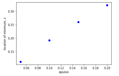
Using your code, use the following command in order to investigate the maxima \((x_m, T_m)\) as \(\epsilon\) varies:
ind = np.argmax(Y[0])
print(ep, z[ind], Y[0, ind])
You may want to consider, as an example, the values \(\epsilon = \{0.05, 0.1, 0.15, 0.2\}\) and fill the following table.
| 0.05 |
0.1122 |
1.5479 |
| 0.1 |
0.1924 |
1.4742 |
| 0.15 |
0.2605 |
1.4094 |
| 0.2 |
0.3226 |
1.3501 |
Create a plot of \((\epsilon, x_m)\) and discuss the observed trend and its implications.
Outer asymptotic solutions
\(\nextSection\)
Begin by setting \[
T = T_{\text{outer}} = T_0(z) + \epsilon T_1(z) + \epsilon^2 T_2(z) + \ldots
\] Substitute the above expansion into the system and solve for the first two orders.
You may verify that the solution is given by
\[\begin{align}
T_0 &= e^{1/2} e^{-z/2}, \\
T_1 &= -\frac{1}{8} e^{1/2} e^{-z/2} (z - 1).
\end{align}\]
Remember: as you solve the outer solution, you impose the boundary condition of \(T(1) = 1\).
Leading-order: at leading order, we get the problem \(2T_0' + T_0 = 0\) subject to \(T_0(1) = 1\). This is solved either by separation of variables or by integrating factor. Using the technique of solving first-order linear equations, (see Chapter 44) we divide, \[
T_0' + \frac{1}{2}T_0 = 0.
\] We then multiply both sides of the equation by \(e^{z/2}\). \[
\frac{\mathrm{d}}{\mathrm{d}z}\Bigl[T_0 e^{z/2}\Bigr] = 0.
\] Integrate, and solve, giving \(T_0 = Ce^{-z/2}\). We now impose \(T_0(1) = 1\) which yields \(C = e^{1/2}\).
First-order: at next order, we get \[
2T_1' + T_1 = -T_0'' \Longrightarrow T_1' + \frac{1}{2}T_1 = -\frac{1}{2}T_0'' ,
\] along with the boundary conditions of \(T_1(1) = 0\).
Again place this into the appropriate form. Again, this is a linear first-order equation. We multiply by the integrating factor \(e^{z/2}\), placing the equation into the form \[
\frac{\mathrm{d}}{\mathrm{d}z} \Bigl[ T_1 e^{z/2} \Bigr] = -\frac{1}{2 }T_0'' e^{z/2} = -\frac{1}{8} e^{1/2}.
\] We integrate once and simplify, yielding \[
T_1(z) = \left(-\frac{e^{1/2}}{8} z + C\right)e^{-z/2},
\] and then impose the condition that \(T_1(1) = 0\). This yields \(C = e^{1/2}/8\) hence \[
T_1(z) = -\frac{e^{1/2}}{8}(z - 1) e^{-z/2}.
\]
Inner asymptotic solutions
\(\nextSection\)
There will be a boundary layer near \(z = 0\). Set \(z = \epsilon^{\alpha} s\) and \(T(z) = U(s)\). Follow the same procedure, as in Chapter 8 in order to determine the correct choice of \(\alpha\) for the inner region. This choice should balance the two terms \(\epsilon T''\) and \(2T'\).
We re-scale \(z = \epsilon^\alpha s\) and let \(T(s) = U(s)\). Then the ODE becomes \[
\epsilon^{1 - 2\alpha} U'' + 2 \epsilon^{-\alpha} U' + U = 0.
\] Balancing the first two terms thus requires that \[
1 - 2 \alpha = -\alpha \Longrightarrow \alpha = 1.
\] Thus the differential equation now becomes \[
U'' + 2 U' + \epsilon U = 0.
\]
Matching and comparison
\(\nextSection\)
Expanding the inner solution as \(U = U_0(s) + \epsilon U_1(s) + \ldots\), write down the equation and boundary conditions that \(U_0\) must satisfy. You will notice that \(U_0\) is governed by a second-order differential equation and therefore needs two boundary conditions. One boundary condition comes from \(z = 0\), i.e. \[
U_0(0) = 0.
\]
The other boundary condition is a matching condition: \[
\lim_{s \to \infty} U_0(s) = \lim_{z \to 0} T_0(z),
\] which imposes that the inner solution, as it leaves the boundary layer, matches the outer solution, it tends into the inner region.
Solve for \(U_0\).
We thus expand \(U = U_0 + \epsilon U_1 + \ldots\). To leading order, we have \[
U_0'' + 2U_0' = 0.
\] Integrating, we find that the general solution is given by \[
U_0(s) = C_1 + C_2 e^{-2s}.
\] We require two boundary conditions. The first condition is given by \(T(0) = 0\) and hence \(U(0) = 0\). The second condition is given by requiring that the inner solution, as \(s \to \infty\), matches the outer solution, as \(z \to 0\). Using our solution above, we find that \[
\lim_{z \to 0} T_0(z) = e^{1/2}.
\] Thus the second boundary condition is \[
\lim_{s \to \infty} U_0(s) = e^{1/2}.
\] Together, both boundary conditions are used to conclude that \[
U_0(s) = e^{1/2}(1 - e^{-2s}),
\] or in terms of \(z\), the inner solution is \[
T_{\text{inner}} \sim e^{1/2}(1 - e^{-2z/\epsilon}).
\]