16 EBM with latitude II

This lecture, we continue our investigation of the latitude-dependent EBM.

Latitude-dependent EBM

Our conservation equation takes the general form for the temperature, $T(y, t)$: \[ C \frac{\partial T}{\partial t} = E_{\text{in}} - E_{\text{out}} + E_{\text{transport}}, \qquad t > 0 \tag{16.1}\] where we shall use the following:

\[ \begin{aligned} E_{\text{in}}(y, t) &= Qs(y)(1 - a(y)), \\ E_{\text{out}}(y, t) &= A + BT, \\ E_{\text{transport}}(y, t) &= k(\bar{T} - T), \end{aligned} \tag{16.2}\]

Our goal is to study the steady-state solutions, $T = T_\infty(y)$, given by solving the implicit equation: \[ T_\infty(y) = \Phi(T_\infty) = \frac{k\bar{T}_\infty + Qs(y)(1 - a(y)) - A}{B + k}. \tag{16.3}\]

We want to know whether other solutions exist with ice lines at $y_s \in [0, 1]$.

16.1 Development of an equation for the ice line

It turns out to be possible to develop an equation for the ice line. First, note from your problem set 5 in Chapter 30, you find that it is possible to solve for the steady-state mean temperature, which we write as $\bar{T}_\infty$. In your problem set, you will develop the following equation by integrating over (Equation 16.1) from $y = 0$ to $y = 1$.

Taking the steady-state limit of (Equation 30.1) this yields \[ \bar{T}_\infty = \frac{Q(1 - \bar{a}) - A}{B}. \tag{16.4}\] The quantity $\bar{a}$ is given by integrating the albedo as follows: \[ \bar{a} = \int_0^1 s(y) a(y) \, \mathrm{d}y = a_i + (a_w {\color{blue}-} a_i)y_s[1 - 0.241 (y_s^2 - 1)], \tag{16.5}\] which is given by (Equation 30.2). You may check that the above formula has the right signs by considering either the complete ice case (ice line at the equator $y_s = 0$) or the complete water/land case (ice line at $y_s = 1$).

Now we return to the implicit equation for the temperature, which is given by (Equation 16.3) and repeated here: \[ T_\infty(y) = \Phi(T_\infty) = \frac{k\bar{T}_\infty + Qs(y)(1 - a(y)) - A}{B + k}. \] Substitute the mean temperature in, and this now yields \[ T_\infty(y) = \frac{Q}{B + k} \left[ s(y) [1 - a(y)] + \frac{k}{B}(1 - \bar{a})\right] - \frac{A}{B}. \tag{16.6}\] This ice line is then found by setting $T = T_C$ at $y = y_s$ in the above formula. Notice, though, that since $s(y)$ is a cubic function, then we would need to solve a cubic equation in general.

16.2 A word about the parameter space

Solutions to our latitude-dependent EBM can be symbolically written as follows: \[ T = T(t, y) = G(y; A, b, k, C, Q, a_i, a_w). \] As you can see, even though it is a relatively simple equation in the sense it is only an ODE in time (and does not involve any spatial derivatives in $y$), is still complicated because the behaviour of the system can depend in a non-trivial way on all the parameters.

You can schematically think of the solution space as a being plotted in 8-dimensional space (or even higher, since the albedo $a$ can be specified more generally). So for instance, bifurcation diagrams can then be plotted for some norm of the solution, say $\bar{T}$ versus the seven other parameters.

There are other representations of the bifurcation diagram(s). For example, you might plot $y_s$ vs $Q$ or $\bar{T}$ vs $A$, and so forth.

16.3 A bifurcation diagram for $Q$ vs $y_s$

Returning to the ice line, we are interested in keeping all other parameters fixed, and then attempting to understand how the ice line evolves as the solar constant $Q$ is changed. For example, we might believe that as $Q$ increases (and hence temperatures rise), the ice line will move towards the North Pole. And as $Q$ decreases, the ice line moves towards the equator.

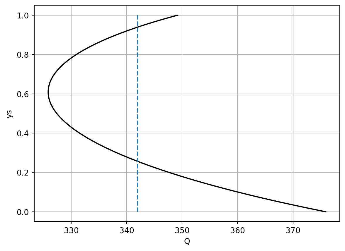
We return to (Equation 16.6) and consider inverting the formulation. For each given ice line location, $y_s \in (0, 1)$, we solve for the $Q$ value. This gives \[ Q = K(y_s) \equiv \frac{\left(T_C + \frac{A}{B}\right)(B + k)}{s(y_s)[1 - \frac{1}{2}(a_i + a_w)] + \frac{k}{B}(1 - \bar{a})}. \tag{16.7}\] Above, we have used the fact that $a(y_s) = \frac{1}{2}(a_i + a_w)$. This can now be plotted in Python, either in the notebook written during lectures, or via the code below.

import numpy as np
import matplotlib.pyplot as plt
A = 202 # outgoing radiation
B = 1.9 # outgoing radiation
k = 1.6*B # transport parameter
s = lambda y: 1 - 0.482*(3*y**2 - 1)/2 # solar weighting
aw = 0.32 # water albedo
ai = 0.62 # ice albedo
Tc = -10.0 # critical temperature for ice formation
Q0 = 342.0 # solar constant (1370 W/m^2 divided by 4)

abar = lambda ys: ai + (aw - ai)*ys*(1 - 0.241*(ys**2 - 1))
Qfunc = lambda ys: (Tc + A/B)*(B+k)/(s(ys)*(1 - (ai+aw)/2) + k/B*(1 - abar(ys)))

# Solve for the ice line
ys = np.linspace(0, 1, 100);
Qs = Qfunc(ys);
plt.plot(Qs, ys, 'k')
plt.plot([Q0, Q0], [0, 1], '--')
plt.xlabel('Q');
plt.ylabel('ys');
plt.grid(1)

On the above graph, we have plotted the reference line, which is at $Q = 342$ W-m-sq. So amazingly, there are two intersections with the black curve, which in fact indicates that two ice lines seem to be possible. One ice line as $y_s$ near $0.95$ and the other has $y_s$ much lower down and near the equator.

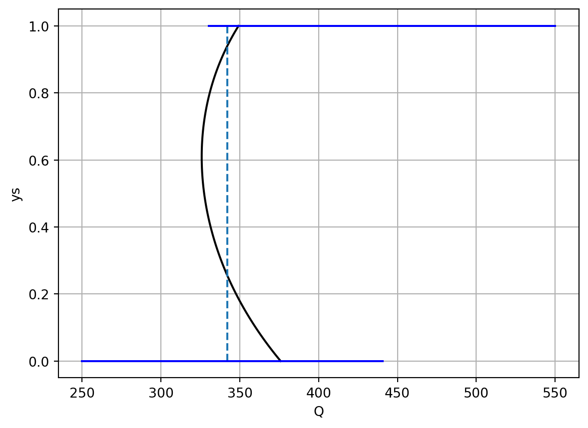
Moreover, the above graph is not complete! When we computed it, we specified that $a(y_s) = \frac{1}{2}(a_i + a_w)$ but this would not be true if there were no ice line, or equivalently if the ice line is located directly at $y = 1$ or $y = 0$. These yield the so-called ice-free states and ice-covered states, respectively.

16.4 Ice-free state

The ice-free state is the state for which $a = a_w = \bar{a}$ for all $y \in [0, 1)$. In this case, the solution can be directly calculated from Equation 16.6. It would then be given by \[ T_\infty(y) = \frac{Q(1 - a_w)}{B + k}\left[s(y) + \frac{k}{B}\right] - \frac{A}{B}. \] This solution has a requirement, which is that when considering the solar constant $Q$, the solar constant cannot be so weak so that an ice line appears for $y < 1$. The minimum value of $Q$ is therefore determined by pinning the ice line right at the North Pole. Thus \[ Q > \frac{(B + k)(T_C + A/B)}{(1 - a_w)[s(1) + k/B]} \approx 330 \mathrm{W} \, \mathrm{m}^{-2}. \] It is of interest to verify that the global mean temperature for a system in this state is a warm $16$ degrees Celsius. According to this model, then, if the mean temperature is above this value, it is possible to have a state where there is no ice anywhere!

16.5 Ice-covered state

A similar argument applies setting $a = a_i = \bar{a}$ for all $y\in (0, 1]$. In this case, \[ T_\infty(y) = \frac{Q(1 - a_i)}{B + k}\left[s(y) + \frac{k}{B}\right] - \frac{A}{B}. \] This time, there is a maximal condition on $Q$ such that any higher value would require an ice line somewhere within the domain, i.e. $y > 0$. Thus \[ Q < \frac{(B + k)(T_C + A/B)}{(1 - a_i)[s(0) + k/B]} \approx 441 \mathrm{W} \, \mathrm{m}^{-2}. \] Again we may verify that this corresponds to a mean temperature of $-38$ degrees Celsius.

import numpy as np
import matplotlib.pyplot as plt
A = 202 # outgoing radiation
B = 1.9 # outgoing radiation
k = 1.6*B # transport parameter
s = lambda y: 1 - 0.482*(3*y**2 - 1)/2 # solar weighting
aw = 0.32 # water albedo
ai = 0.62 # ice albedo
Tc = -10.0 # critical temperature for ice formation
Q0 = 342.0 # solar constant (1370 W/m^2 divided by 4)

Qmin = ((B+k)*(Tc + A/B))/((1-aw)*(s(1)+k/B)) 
Qmax = ((B+k)*(Tc + A/B))/((1-ai)*(s(0)+k/B))
print("Minimal Q for ice-free state = ", Qmin)
print("Max Q for ice-covered state = ", Qmax)

# Note version in lectures was a 1/2 factor off on the second grouping of terms; 
# now corrected to match Q6 of PS4
abar = lambda ys: ai + (aw - ai)*ys*(1 - 0.241*(ys**2 - 1))
Qfunc = lambda ys: (Tc + A/B)*(B+k)/(s(ys)*(1 - (ai+aw)/2) + k/B*(1 - abar(ys)))

# Solve for the ice line
ys = np.linspace(0, 1, 100);
Qs = Qfunc(ys);
plt.plot(Qs, ys, 'k')
plt.plot([Q0, Q0], [0, 1], '--')
plt.plot([250, Qmax], [0, 0], 'b')
plt.plot([Qmin, 550], [1, 1], 'b')
plt.xlabel('Q');
plt.ylabel('ys');
plt.grid(1)

Minimal Q for ice-free state =  330.3616063989335
Max Q for ice-covered state =  440.72694936919913

16.6 Partially ice-covered states

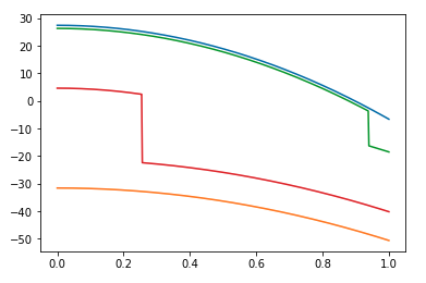
In lectures, we demonstrated, that there are four possible solutions of the latitude EBM. Two of the solutions, developed above, correspond to completely covered ice-state and ice-free states. The other two solutions are partially-iced states.

Figure 16.1: The four possible solutions; orange and blue show the completely-ice and ice-free states; red and green show the partial ice-covered state. These are shown for $A = 202$, $B = 1.9$, $k = 1.6 B$, and $Q$ = 342$