12  EBM with nonlinear albedo

Recall that we previously introduced the basic energy balance model in Chapter 4. There, we derived the basic heat equation model (Equation 4.7) for the Earth’s temperature given by the following ordinary differential equation (ODE) for $T=T(t)$,
$$\begin{array}{}\text{(12.1)}& C\frac{\mathrm{d}T}{\mathrm{d}t}=Q(1-a)-\sigma \gamma T^4,\end{array}$$ where we have defined $C=\rho c_{p}d$ as the heat capacity of the atmosphere. Above, the solar flux, Q is often taken to be $Q=1370/4=342$ W/m², $\sigma =5.67\times {10}^{-8}$ W/(m²K⁴), and $\gamma \le 1$ is the greenhouse gas factor.

In this chapter, we discuss the effects of considering a nonlinear albedo, $a=a(T)$, as well as some of the numerical and analytical tools at our disposal for studying the above equation.

12.1 Steady-state analysis

Below, we shall let $T=T_{\mathrm{\infty }}$ be the steady-state solution that is independent of time. Whenever convenient, we will drop the subscript notation and simply refer to the steady state as $T$.

Previously, we have assumed that the planetary albedo, $a$, is constant and independent of temperature. In actuality, water can turn to snow and ice and vice versa; since snow and ice have much higher albedo than open water, then we should consider $a=a(T)$.

Let us assume that there are two relevant ranges to consider: T < 150K (cold) and T > 280K (hot). Let us assume that the albedo is, in these two regions: $$a(T)\approx \{\begin{array}{ll}0.7& \mathrm{if}T<150\mathrm{K},\\ 0.3& \mathrm{if}T>280\mathrm{K}.\end{array}$$ The above guarantees that more energy is reflected if temperatures are low. To model this process, we can use a ramp function to specify the albedo over all temperatures: $$\begin{array}{}\text{(12.2)}& a(T)=A-B\tanh (k(T-265)).\end{array}$$ where $A=0.5$, $B=0.2$, $k=0.1$, and $T_0=265\mathrm{K}$. Recall that the tanh function is given by $$\tanh (x)=\frac{\sinh (x)}{\cosh (x)}=\frac{e^x-e^{-x}}{e^x+e^{-x}}.$$

Let us further assume that the system is in steady state, so that the temperature is determined by solving the equation $$\begin{array}{}\text{(12.3)}& f(T)=Q[1-a(T)]-\sigma \gamma T^4=0.\end{array}$$

In the following code, we plot the two terms that make up $f$, and their intersections indicate roots of $f=0$. We then use the Python ‘fsolve’ function to approximate the roots given initial guesses.

import numpy as np
import matplotlib.pyplot as plt
import scipy.optimize as sciopt

Q = 342
sigma = 5.67e-8 
gamma = 0.62

TT = np.linspace(220,310,50)

def fun(T):
    a = 0.5 - 0.2*np.tanh((T - 265)/10)
    x = (1-a)*Q
    return x
LHS = fun(TT)

plt.plot(TT, LHS)
plt.plot(TT, gamma*sigma*TT**4, 'k--')

def eq(T):
    x = fun(T) - gamma*sigma*T**4
    return x
T1 = sciopt.fsolve(eq, 230)
T2 = sciopt.fsolve(eq, 265)
T3 = sciopt.fsolve(eq, 290)
print("T1 = {:.2f}".format(T1[0]))
print("T2 = {:.2f}".format(T2[0]))
print("T3 = {:.2f}".format(T3[0]))

T1 = 232.55
T2 = 265.56
T3 = 286.74

Therefore multiple equilibria are observed.

12.2 Bifurcation diagram

$$

During the lectures, the above script plotting the steady-state solutions will be examined in order to understand the effects of changing $Q$.

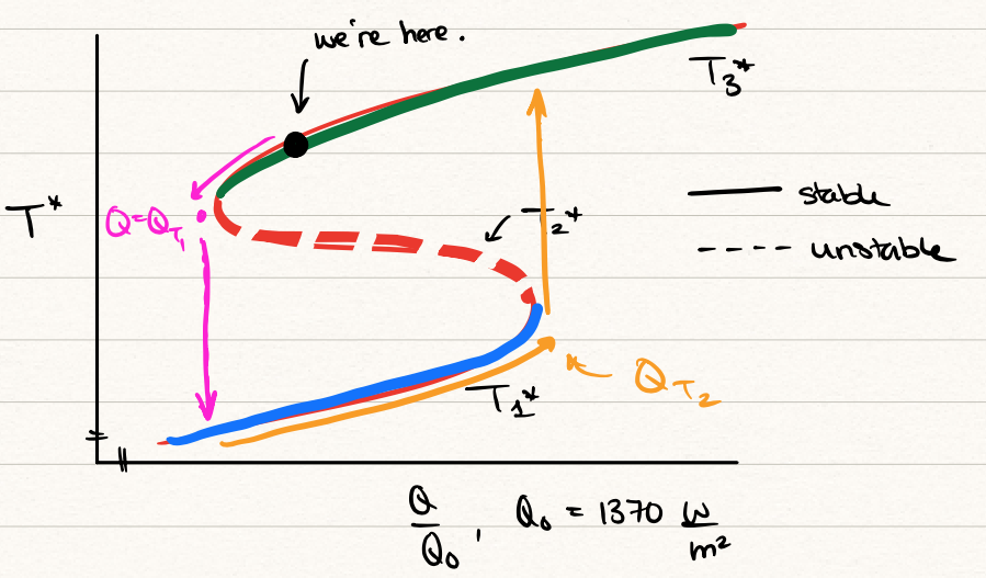
It will be observed that dependent on the solar radiation, there may be one or three steady-state solutions. This leads to the following key bifurcation diagram.

Figure 12.1: Bifurcation diagram of $Q/Q_0$ vs $T_{\mathrm{\infty }}$

We noted the following:

• The system has three steady states, given by the green, red, and blue curves.
• The middle state is unstable (shown dashed).
• The system exhibits hysteresis. Note that if we decrease $Q/Q_0$ past the tipping point, marked $Q_{T1}$ in the image, then we would evolve to the lower stable steady state (which is the ice state). However, while we are in the ice stated, if we were to attempt to increase the solar radiation to return to the green branch, we would need to arrive at $Q_{T2}$ to do so; this irreversibility is known as hysteresis. ## Dynamics and phase line solutions

The full time-dependent model is given by $$C\frac{\mathrm{d}T}{\mathrm{d}t}=f(T),$$ so we may use the positivity or negativity of $f$ in order to sketch the time-dependent behaviour of the system.

To see this, we can perform an asymptotic analysis near the fixed points. Let the initial condition be considered near the fixed point: $$T(t=0)=T_{\mathrm{\infty }}+\delta ,$$ where $\delta \ll 1$. Then we expand the solution into an asymptotic expansion, $$T(t)=T_{\mathrm{\infty }}+\delta T_1(t)+\delta T^2(t)+\dots$$ Substitution into the above ODE gives, at $O(\delta )$, $$C\frac{\mathrm{d}{T}_1}{\mathrm{d}t}=f^{\prime }(T_{\mathrm{\infty }})T_1,$$ and hence, with $T_1(0)=1$, we have $$T_1(t)=e^{f^{\prime }(T_{\mathrm{\infty }})t/C}.$$ Therefore, depending on the positivity or negativity of the gradient function, the perturbation will either decay or grow as $t\to \mathrm{\infty }$.

It can then be verified that the centre equilbria is unstable while the other two are stable. The higher temperature corresponds to the one that the Earth is currently in, but according to this model, there seems to be the possibility of a colder climate (50 degrees colder) where the Earth is entirely covered with snow and ice.

Interestingly, there is some evidence that the Earth’s climate may have been in this so-called state up to four times between 750 million and 580 million years ago (Neoproterozoic age). Observations of geological deposits suggest that the Earth has undergone periods of complete global glaciation where there have been very minimal biological activity. During this period, there is a massive build-up of CO₂ in the atmopshere, leading to huge greenhouse effect. As $\gamma$ decreases in our model, the equilibrium can then shift, suddenly transitioning the Planet into the warm state.

12.3 Re-scaling and Budyko’s model

$$

To model the outgoing radiation, we use the quartic Stefan-Boltzmann law. However, over the range of temperatures we are interested-in, it seems that a simpler approximation is sufficient. In your homework, you will investigate the re-scaling and shifting of temperature, such that $$T=T_0+[T]\tilde{T},$$ where $T_0=265\mathrm{K}$. Then under the assumption that temperatures are not-so-far from $T_0$, we expand $$(T_0+[T]\tilde{T}{)}^4\sim T_0^4+4T_0^3[T]\tilde{T}=C_1+C_2\tilde{T}.$$ This simplifies the model considerably.

This is, in fact, a theoretical justification of Budyko’s model, first suggested by Budyko (Budyko 1969), where instead of the Stefan-Boltmann law that provides the cumbersome quartic power of $T$, we use instead $$E_{\text{out}}=\sigma \gamma T^4\approx A+BT,$$ where $A$ and $B$ will vary with location and climate. For instance, for the Northern Hemisphere, (Kaper and Engler 2013) gives the values of $A=203.3{\text{Wm}}^{-2}$ and $B=2.09{\text{Wm}}^{-2}{\text{deg}}^{-1}$ and where temperature is measured in degrees Celcius. As shown above, one can interpret this as a linear expansion of the Stefan-Boltzmann law (after which similar values of $A$ and $B$ are derived).

The above Budyko model will be a staple of the latitude-dependent model introduced in the next chapter.

Budyko, Mikhail I. 1969. “The Effect of Solar Radiation Variations on the Climate of the Earth.” Tellus 21 (5): 611–19.

Kaper, H., and H. Engler. 2013. Mathematics and Climate. SIAM.