Section7.2Boundaries, surfaces and interfaces of fluids
This movie shows an experiment in which two dye streaks illustrate the motion of a viscous fluid. As can be seen:
The end of dye streak at the solid wall does not move relative to the wall. This motivates the no slip condition at a solid–fluid boundary Definition 7.2.1.
The two dye streaks on either side of the fluid–fluid interface move together, illustrating that the velocity is continuous across a fluid–fluid interface Definition 7.2.4.
are satisfied. This condition on the velocity components is called the no-slip condition. When solving problems in fluid mechanics we usually apply these relationships to provide boundary conditions.
Note that this condition is weaker than the corresponding one for viscous fluids, since it only applies to one component of the velocity. As we will shortly see, the extra conditions for viscous fluids are mathematically necessary, since the equation for conservation of momentum for viscous fluids has spatial derivatives of higher order.
Subsection7.2.2Force balance at the boundary/interface
In addition to the boundary conditions on the velocity given in Subsection 7.2.1, we sometimes need to apply a force balance condition at the boundary of the fluid or at the interface between two fluids in a free boundary problem.
Thankfully, in the case of a fluid–solid boundary, if the solid is rigid (which we often assume), the no-slip boundary conditions on the velocity are sufficient to solve the problem mathematically. If desired, a force balance can be performed after solving the problem, and this determines the stress (force per unit area) that the fluid exerts on the solid wall, and we can thus find the reaction force that the wall applies in order to maintain its position in the presence of the flowing fluid.
However, if the solid moves in response to the fluid, either because it is an elastic solid or because the solid is not tethered, then a force balance is required to solve the problem mathematically. This is called a fluid–structure interaction problem, and these are typically very difficult to solve.
Furthermore, at a fluid–fluid interface, a force balance is typically required to solve the problem. The difference between the stresses of the two fluids on the interface (the forces each fluid exerts on the interface per unit area of the interface) is balanced by the surface tension that arises within the interface.
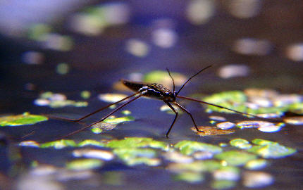
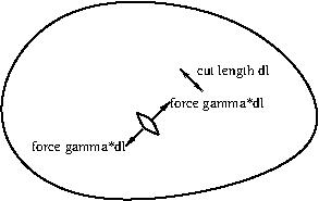
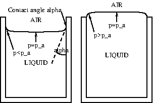
The interface between two immiscible fluids (e.g. air and water, or water and mercury) creates surface tension, a force per unit length. This is of considerable importance in many fluid mechanics problems, especially those involving small lengthscales.
A spherical fluid droplet of radius \(R\) has coefficient of surface tension \(\gamma\text{.}\) What is the pressure difference between the inside and outside of the droplet?
\begin{equation*}
\Delta p = p_{\textrm{in}} - p_{\textrm{out}} = \frac{2\gamma}{R}.
\end{equation*}