Exercises

Exercises 4.7 Exercises

There is an excellent website at www.potentialflows.com that allows you to plug in different flow elements (sources/sinks, vortices, etc.) into a potential flow and observe the streamlines and potential-flow lines. In your exercises, use this to help you visualise the flow.

🔗

Remark 4.7.1. 2025-26 note.

After having administered this problem set, we realised how long it was! It was not our intention to make the exercises too long, but we had wanted to make sure you had plenty of examples of potential flows and conformal maps.

🔗

To aid your studying, we would highlight the following exercises that might be prioritised:

Q1. Basic calculations is useful to do a few to learn the ins and outs, though note it does become tedious. I would suggest on first attempt to ignore the request to calculate fluid forces.
🔗

🔗
Q2. This is nice to do. It teaches you that much of the "pain" of Q1 can be handled by the streamfunction theorem.
🔗

🔗
Q4 and Q5 can be covered on the first pass. These are quick and get you practice on method of images.
🔗

🔗
Q9 and Q10 can be done on a first pass. Q10 was done almost entirely in lectures but students can use this to go through the ideas.
🔗

🔗

🔗

Potential flows, part 1.

These exercises cover approximately around sections 4.1 (the velocity potential) to 4.3 (the complex potential).

🔗

1. Basic calculations.

The following question relates to two-dimensional potential flow. Remember that the fluid flux through a surface given by contour \(C\) is given by (2.2.2), or

\begin{equation*} \int_C \bu \cdot \bn \, \de{s}. \end{equation*}

You will get some practice on calculating this quantity below.

🔗

We can also calculate the total force on the surface specified by \(C\) by using the integral in (2.2.3). Since the force in potential flow is given by Theorem 3.3.2, then the total force is

\begin{equation*} \text{total force} = \int_C (-p\bn) \, \de{s} \end{equation*}

where \(p\) is the pressure force given by Bernoulli’s equation:

\begin{equation*} p = p_0 - \frac{\rho}{2} |\bu|^2, \end{equation*}

and \(p_0\) is a reference value and we ignore gravity.

🔗

For each of the following elementary flows, state or calculate:

the complex potential, \(f(z)\text{;}\)
🔗

🔗
the velocity vector, written in vector form \(\bu = [u, v]\text{;}\)
🔗

🔗
the flux and fluid force on a surface consisting of a circle of unit radius;
🔗

Hint: the unit normal for the circle is \(\bn = [\cos\theta, \sin\theta]\text{;}\) when converting to polar coordinates remember that \(\de{s} = r\de{\theta}\text{.}\)
🔗

🔗
the flux and fluid force on a surface consisting of a plate given by the line \(y = -x + 1\) with \(0 \leq x \leq 1\text{.}\)
🔗

🔗

🔗

(a)

Uniform flow of velocity \(U\) oriented at an angle of \(\pi/4\) to the horizontal.

🔗

Solution.

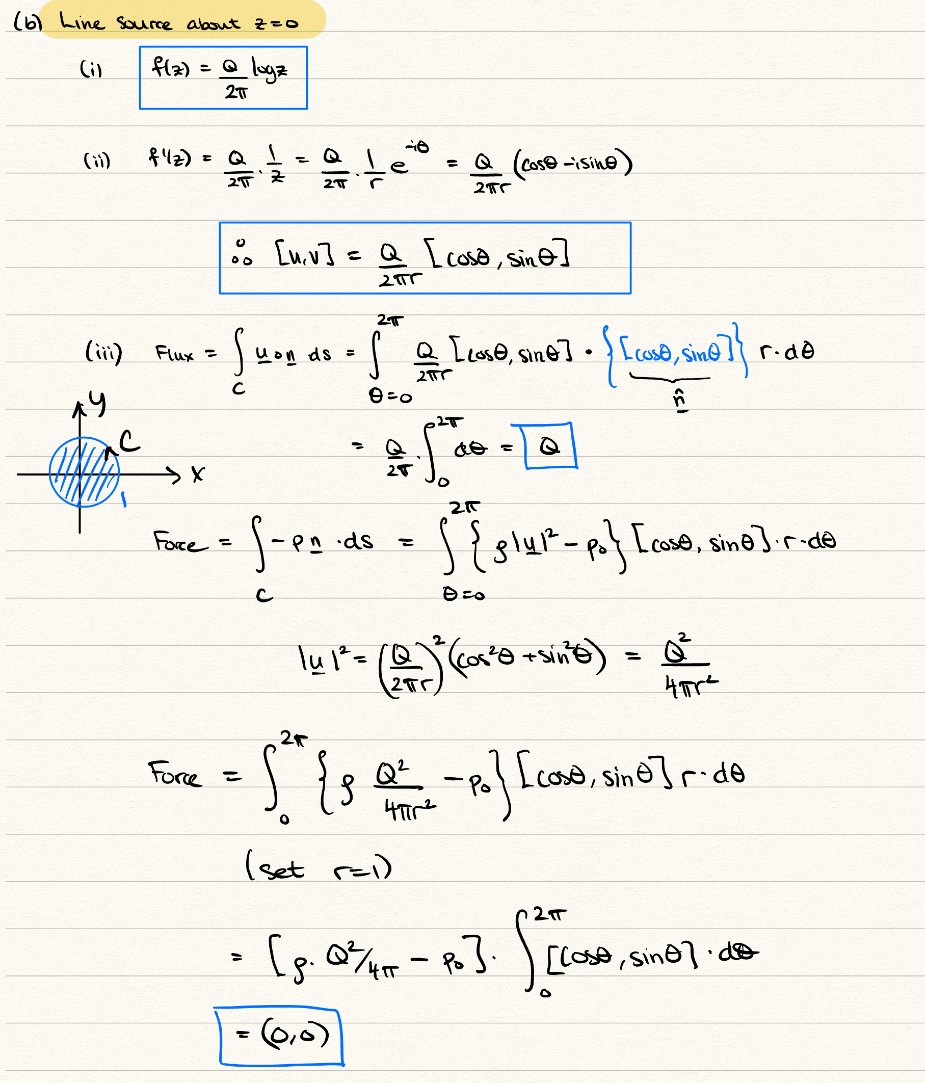
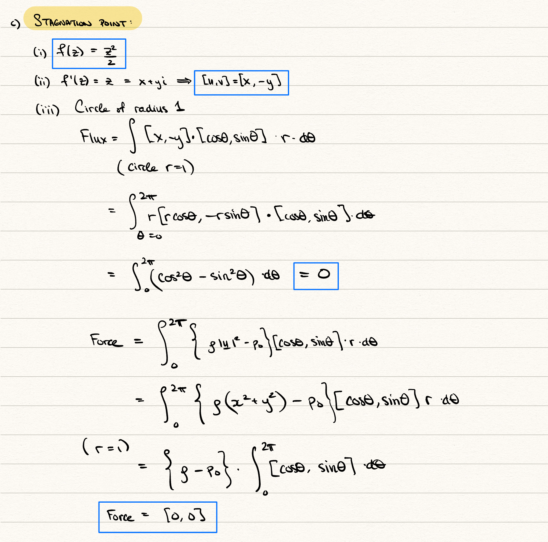
(i) complex potential given in the notes is

\begin{equation*} f(z) = U\e^{-\im\alpha}z = U\e^{-\im \pi/4}z\text{;} \end{equation*}

🔗

(ii) complex velocity is given by \(f'(z) = u - \im v = U\e^{-\im \pi/4}\text{.}\) Writing out the velocity components in vector form, we have

\begin{equation*} \bu = U \Bigl[ \cos(\pi/4), \, \sin(\pi/4) \Bigr] = U \frac{\sqrt{2}}{2} \Bigl[1, 1\Bigr]. \end{equation*}

🔗

(iii) We expect the flux past a circle will be zero (since the flow will enter one side and exit the other). The flux is given by

\begin{equation*} \int_{r = 1} \bu \cdot \bn \, \de{s} = U\frac{\sqrt{2}}{2} \int_0^{2\pi} [1, 1] \cdot [\cos\theta, \sin\theta] \de{\theta} = 0. \end{equation*}

🔗

The force is given by

\begin{equation*} \bF_{\text{total}} = \left(\frac{\rho}{2} U^2 - p_0\right) \int_0^{2\pi} [\cos\theta, \sin\theta] \, \de{\theta} = [0, 0]. \end{equation*}

The total force again is zero since the force on the two hemispheres will cancel themselves out.

🔗

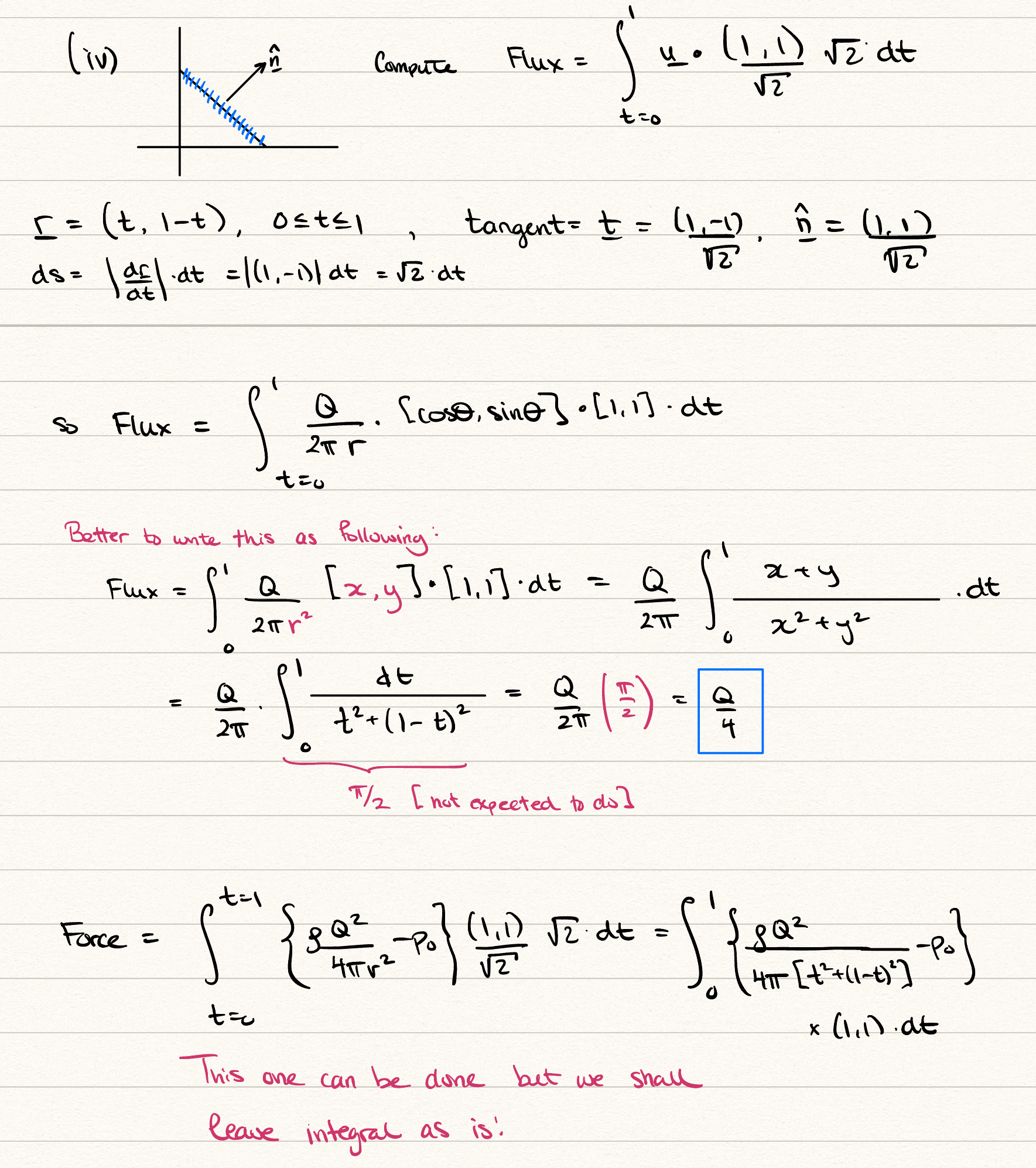
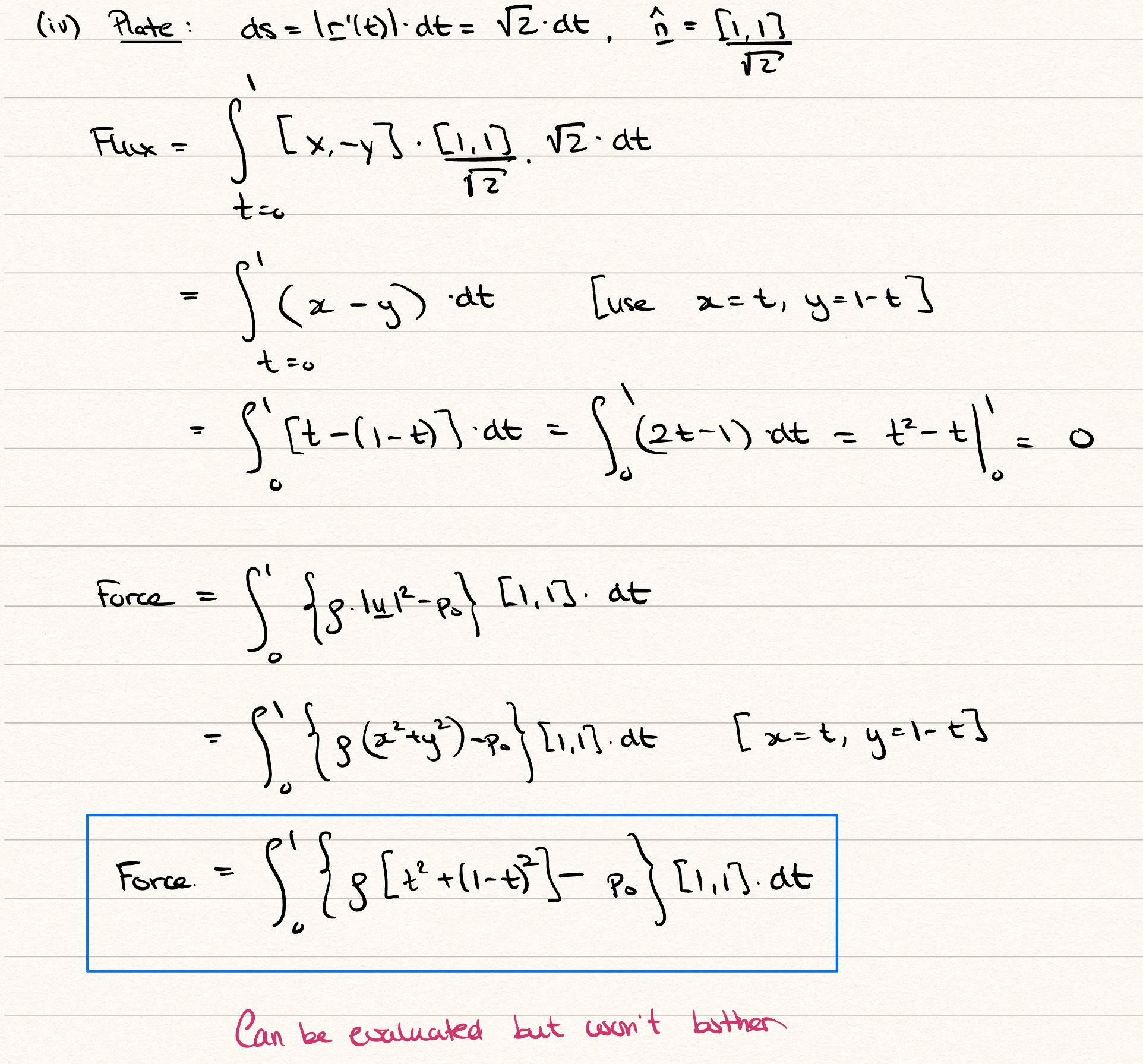
(iv) The normal of the plate is given by

\begin{equation*} \bn = \frac{[1, 1]}{\sqrt{2}} \end{equation*}

(here we assume this normal is pointing ’out’). We can parameterise the plate using a vector equation for the position vector:

\begin{equation*} \br(t) = [t, -t + 1], \quad 0 \leq t \leq 1, \end{equation*}

since the equation of the line is \(y = -x + 1\text{.}\) Then

\begin{equation*} |\br'(t)| = |[1, -1]| = \sqrt{2}. \end{equation*}

So the surface conversion is

\begin{equation*} \de{s} = |\br'(t)| \, \de{t} = \sqrt{2} \de{t}. \end{equation*}

The flux is then

\begin{equation*} U\frac{\sqrt{2}}{2} \int_{t = 0}^1 \frac{[1, 1]}{\sqrt{2}} \cdot [1, 1] \sqrt{2} \de{t} = \sqrt{2}U. \end{equation*}

The above makes perfect sense. The fluid is entirely normal to the plate, and the plate has length \(\sqrt{2}\text{.}\)

🔗

For the force, remember that the pressure is constant, since the speed is constant. Thus

\begin{equation*} \bF_{\text{total}}= \left(\frac{\rho}{2}U^2 - p_0\right) \int_0^1 \frac{[1, 1]}{\sqrt{2}} \cdot \, \sqrt{2} \, \de{t} =\left(\frac{\rho}{2}U^2 - p_0\right) [1, 1]. \end{equation*}

🔗

(b)

A line source of strength \(Q\) located at the origin.

🔗

Solution.

The part about integrating the flux and forces for the little diagonal plate segment has some annoy integrals. You are not expected to obtain the final values of the integrals, but you will see in the next question that they can be predicted rather easily using a theorem about the streamfunctions.

🔗

(c)

Stagnation point flow with a stagnation point at the origin.

🔗

Solution.

The integrals for the flux and force on the plate are less annoying than in the previous geometries, but again we have left the final force calculuation un-evaluated (out of laziness).

🔗

(d)

A line vortex flow of strength \(\Gamma\) placed at the origin.

🔗

Solution.

🔗

2. Evaluation of the flux.

Return to the previous question and, instead of directly calculating the flux via a line integral, use Theorem 4.2.3 to calculate the flux for the two geometries (unit circle and straight plate) for each of the flows given.

🔗

Solution.

This is a nice question to do because there is a simple recipe. For each of the complex potentials in the previous question, find the imaginary part to obtain the streamfunction. Then evaluate the difference in streamfunction values at the start and end values of the desired curve.

🔗

For uniform flow, \(\psi(r, \theta) = Ur \sin(\theta - \alpha)|\text{.}\) For the case of a circle, the flux is:

\begin{equation*} |\psi(1, 2\pi) - \psi(1, 0)| = 0. \end{equation*}

For the case of a plate,

\begin{equation*} |\psi(1, 0) - \psi(1, \pi/2)| = U|\sin(-\pi/4) - \sin(\pi/4)| = \sqrt{2}U. \end{equation*}

🔗

For source flow, \(\psi = (Q/2\pi) \theta\) once you convert the logarithm into its real and complex parts. Then for the circle:

\begin{equation*} |\psi(1, 2\pi) - \psi(1, 0)| = Q. \end{equation*}

For the case of the plate,

\begin{equation*} |\psi(1, 0) - \psi(1, \pi/2)| = \frac{Q}{4}. \end{equation*}

(Actually calculating the above might convince you the route of calculating flux by integrals is possible!).

🔗

For the stagnation point, \(\psi = (r^2/2)\sin 2\theta\text{.}\) For the circle,

\begin{equation*} |\psi(1, 2\pi) - \psi(1, 0)| = 0. \end{equation*}

For the case of the plate,

\begin{equation*} |\psi(1, 0) - \psi(1, \pi/2)| = 0. \end{equation*}

🔗

For the case of the line vortex, \(\psi = -\Gamma/(2\pi)\log r\text{,}\) and for the circle,

\begin{equation*} |\psi(1, 2\pi) - \psi(1, 0)| = 0, \end{equation*}

while for the plate,

\begin{equation*} |psi(1, 0) - \psi(1, \pi/2)| = 0. \end{equation*}

🔗

3. Doublet.

A line source of strength \(Q\) is at \(z = a\) and a line sink of the same strength is at \(z = -a\) where \(a > 0\text{.}\)

🔗

(a)

Write down the complex potential, \(f(z)\text{.}\) Find \(f'(z)\text{.}\) Locate any stagnation points and derive an equation for the streamlines of the flow. Finally, use a plotter, such as the one at the potential flow simulator to sketch the streamlines.

🔗

Answer.

The complex potential is the sum of a line source and line sink:

\begin{equation*} f(z) = \frac{Q}{2\pi} [\log(z - a) - \log(z + a)]. \end{equation*}

Therefore the complex velocity is given by

\begin{equation*} f'(z) = \frac{Q}{2\pi} \left[ \frac{1}{z-a} - \frac{1}{z+a}\right]. \end{equation*}

Stagnation points are where \(f'(z) = 0\text{.}\) There are no stagnation points. The streamfunction is given by

\begin{equation*} \Im f = \frac{Q}{2\pi}(\theta_1 - \theta_2), \end{equation*}

where \(\theta_1\) and \(\theta_2\) are angles measured relative to the positions about \(\pm a\text{.}\) Thus,

\begin{equation*} \theta_{1,2} = \tan^{-1} \left( \frac{y}{x \mp a} \right). \end{equation*}

The streamlines are given where \(\psi\) is constant. The streamlines are shown below.

🔗

Almost doublet — Figure 4.7.2. Streamlines for a sink and source
🔗

🔗

(b)

Let \(a \to 0\) and \(Q \to \infty\) while keeping the product \(aQ\) fixed. This gives the flow due to a doublet. Show that its complex potential is \(\mu/z\) where \(\mu\) is expressed in terms of \(a\) and \(Q\text{.}\) It will be useful for you to use the fact that

\begin{equation*} \log(1 + \alpha) = \alpha + O(\alpha^2) \end{equation*}

considered as an appropriate approximation when \(\alpha\) is small. Show that the streamlines are circles through the origin with centres on the \(y\)-axis.

🔗

Solution.

Expanding the logarithms for small \(a\) gives

\begin{equation*} \log z - \log z + \log(1 - a/z) - \log(1 + a/z) \sim -\frac{2a}{z}. \end{equation*}

Thus in the limit \(a \to 0\text{,}\) we have

\begin{equation*} f(z) \sim -\frac{Qa}{\pi} \frac{1}{z}. \end{equation*}

Therefore, we let both \(a \to 0\) and \(Q \to \infty\) in a fashion such that \(m = aQ\) is fixed. We then have the potential

\begin{equation*} f(z) = \frac{\mu}{z} \end{equation*}

where \(\mu = -Qa/\pi.\)

🔗

Potential flows, part 2.

These exercises will cover the second part of Chapter 4, from sec. 4.4 (the method of images).

🔗

4. Single source in a semi-infinite flow.

Verify that a single source of strength \(Q\) placed at the point \(z = d > 0\) is insufficient to describe flow bounded in the semi-infinite region, \(x > 0\text{,}\) with a planar boundary at \(x = 0\text{.}\) What is the horizontal and vertical velocities on the boundary? Find an equation for the streamlines and sketch the flow.

🔗

Solution.

🔗

5. A source in a semi-infinite flow.

Consider the situation of two point sources of identical strength, \(Q\text{,}\) placed at \(z = \pm d\text{,}\) with \(d \gt 0\text{.}\) Develop equations for the complex potential, \(f(z) = \phi + \im \psi\text{,}\) and complex velocity, \(u - \im v\text{.}\)

🔗

Demonstrate that the streamlines are given by hyperbolae and develop the equation for their form.

🔗

Solution.

🔗

6. Two vortices and a dividing boundary.

Consider the situation of two point vorticies of identical strength, but opposite direction, placed at \(z = \pm d\text{,}\) with \(d \gt 0\text{.}\) Develop equations for the complex potential, \(f(z) = \phi + \im \psi\text{,}\) and complex velocity, \(u - \im v\text{.}\)

🔗

Demonstrate that the streamlines are given by

\begin{equation*} \psi = \frac{\Gamma}{2\pi}\log \left( \frac{r_2}{r_1}\right). \end{equation*}

🔗

Solution.

🔗

7. A line source in a flow; stagnation points.

Incompressible inviscid fluid occupies the region \(y > 0\text{,}\) and there is a rigid plane wall at \(y = 0\text{.}\) There is a uniform flow, speed \(U\text{,}\) in the positive \(x\)-direction, and a line source of strength \(Q\) at \((0, a)\text{,}\) where \(a > 0\text{.}\) Find the complex potential \(f(z)\) and calculate \(f'(z)\text{.}\) Let \(\beta = Q/(2\pi aU)\text{.}\) Show that if \(\beta > 1\) there are two stagnation points, both on the wall, while if \(\beta < 1\) there is only one, in the fluid, a distance \(a\) from the origin. Try to sketch the streamlines in either case

🔗

Solution.

The potential is given by

\begin{equation*} f(z) = Uz + \frac{Q}{2\pi} [\log(z - a\im) + \log(z + a\im)] = Uz + \frac{Q}{2\pi} \log(z^2 + a^2). \end{equation*}

The complex velocity is then

\begin{equation*} f'(z) = U + \frac{Qz}{\pi(z^2 + a^2)}. \end{equation*}

🔗

A stagnation point requires \(f'(z) = 0\) and so we solve the resultant quadratic to obtain

\begin{equation*} z = \frac{-Q \pm \sqrt{Q^2 - (2a\pi U)^2}}{2\pi U}. \end{equation*}

Setting \(\beta = Q/(2\pi a U)\text{,}\) there are two real roots if \(\beta > 1\text{.}\) Hence this is the case of two stagnation points along the axis. If \(\beta < 1\text{,}\) then there two complex conjugate points, and hence only one stagnation point in the flow field.

🔗

🔗

8. The exponential and sinusoidal conformal maps.

Check where each of the labeled points in the associated diagrams for the exponential map (4.5.4) and (4.5.5) are sent, from the \(z\)-plane to the \(\zeta\)-plane. In each of these cases, verify that an interior (within the fluid domain) is sent to the upper half-plane.

🔗

Construct the complex potential that corresponds to a single line source placed within the fluid in each of these cases (an infinite strip of height \(h\) and a semi-infinite strip).

🔗

Solution.

For the exponential map, \(\zeta = \e^{\pi z/h}\text{,}\) we want to check the outputs of points A, B, C, D listed on the figure. These are as follows.

🔗

Table 4.7.5. Exponential map

🔗

\(z\)-plane	\(\zeta\)-plane
\(-\infty + \im h\)	\(0^-\)
\(\infty + \im h\)	\(-\infty\)
\(\infty\)	\(+\infty\)
\(-\infty\)	\(0^+\)

When thinking of the map, the most important step is to just verify that the line, \(z = t + \im h\text{,}\) is mapped to \(\zeta = -\e^{\pi t/h}\text{,}\) so the effect of shifting vertically by \(\im h\) is to negate the values as compared to evaluating on \(z = t\text{.}\) To verify the region the fluid is in, simply "walk" from ABCD in the \(z\)-plane, and remark on the orientation of the fluid relative to your journey (the fluid is on the right). The direction is preserved also in the \(\zeta\)-plane.

🔗

The potential that corresponds to a single source is found by using method of images in the \(\zeta\) plane and mapping backwards. It is

\begin{align*} F(\zeta) \amp= \frac{Q}{2\pi} \left[\log(\zeta - d) + \log(\zeta + \overline{d})\right], \\ f(z) \amp= \frac{Q}{2\pi} \left[\log(\e^{\pi z/h} - d) + \log(\e^{\pi z/h} + \overline{d})\right], \end{align*}

🔗

For the trigonometric map, \(\zeta = \sin(\pi z/2a)\text{,}\) the work is similar.

🔗

Table 4.7.6. Trigonometric map

🔗

\(z\)-plane	\(\zeta\)-plane
\(-a + \im \infty\)	\(-\infty\)
\(-a\)	\(-1\)
\(0\)	\(0\)
\(a\)	\(1\)
\(a + \im \infty\)	\(\infty\)

The potential that corresponds to a single source is found by using method of images in the \(\zeta\) plane and mapping backwards. It is

\begin{align*} F(\zeta) \amp= \frac{Q}{2\pi} \left[\log(\zeta - d) + \log(\zeta + \overline{d})\right], \\ f(z) \amp= \frac{Q}{2\pi} \left[\log(\sin(\pi z/2a) - d) + \log(\sin(\pi z/2a) + \overline{d})\right], \end{align*}

🔗

9. Elementary conformal maps.

Define the term conformal map.

🔗

Write down the conformal maps from the wedge \(0 < \textrm{arg}(z) < \alpha\) into the upper half-plane. Find all the points at which the map is not conformal.

🔗

Solution.

A conformal map is a mapping \(\zeta = g(z)\) where \(g\) is analytic and its derivative is nonzero in some region of the complex plane.

🔗

The map from the wedge to the upper half-plane is given in the notes near (4.5.1). It is \(\zeta = z^{\pi/\alpha}\text{.}\) The points where the mapping is not conformal are the critical points listed in the figure Figure 4.5.2. Point A at infinity is mapped directly to +infinity. The origin is mapped to the origin. And the point, B, found via \(z = r\e^{\im\alpha}\text{,}\) is sent to \(\zeta = -r^{\pi/\alpha}\) and then afterwards \(r \to \infty\text{.}\)

🔗

10. Flow past a flat plate.

Show that the circle \(|\zeta| = a\) is mapped to a line segment

\begin{equation*} S = \{ z: \Im z = 0, -2a \leq \Re z \leq 2a\} \end{equation*}

along the real \(z\)-axis by the Joukowski transformation

\begin{equation*} z = \zeta + \frac{a^2}{\zeta}. \end{equation*}

🔗

Deduce that the exterior of the line segment is mapped to the exterior of the circle \(|\zeta| = a\) by the transformation

\begin{equation*} \zeta = \frac{1}{2}\left( z + \sqrt{z^2 - 4a^2}\right). \end{equation*}

Carefully define the function \(\sqrt{z^2 - 4a^2}\) and determine where the mapping above is conformal.

🔗

Constuct a flow, by providing the complex potential \(\phi + \im \psi\) that consists of the following elements: (i) uniform flow oriented an angle \(\alpha\) to the horizontal at infinity; (ii) a line source of strength \(Q\) placed in the flow; and (iii) a horizontal flat plate of length \(2a\) on the axis, \(-2a < z < 2a.\)

🔗

Sketch what you believe will be the streamlines of such a flow.

🔗

Solution.

This problem was covered in the Week 5, Lecture 2 set, so do have a look at the video recordings to remind yourself. But is essentially broken up as follows. First, verify that there is a map from the outside of the circle (in \(\zeta\)) to a flat plate (in \(z\)).

🔗

Next, make sure the function \(z = f(\zeta)\) is well defined via specification of the branch structure.

🔗

Finally, construct a generic map of uniform flow plus a source, called \(F(\zeta)\text{.}\) Use the circle map theorem to obtain the corresponding flow past a circular cylinder with radius \(a\text{.}\) Finally use your connection to \(z\) to get the final solution.

🔗

11. The Magnus effect and flow past a circular cylinder.

During the problem class, we will study Example 4.6.5 corresponding to verifying different properties of uniform flow past a circular cylinder, ending with studying the Magnus effect due to adding an initial line vortex of strength \(\Gamma\) into the flow. Please review the derivations and make your own notes on the example so that you are confident with the problem and its conclusions.

🔗

Solution.

There is no solution needed since you are asked just to review what is already written in the notes in Example 4.6.5.

🔗

Prev Top Next