Logo image

Section 6.2 The Helmholtz vortex theorems

In this section, we cover some important theorems governing the motion of vortices in a fluid flow.
Helmholtz
Figure 6.2.1. Hermann von Helmholtz (1821-1894)

Subsection 6.2.1 The theorems

Proof of the Helmholtz vortex theorems.

Proof of the first vortex theorem. For a given vortex line, choose two vortex surfaces containing the line such that the vortex line is the intersection of the two vortex surfaces.
Choose a closed curve \(C\) lying within one the vortex surfaces. The circulation around \(C\) is
\begin{equation*} \Gamma=\oint_C\bu\cdot\de\bx=\iint_S\bomega\cdot\bn\,\de S, \end{equation*}
where the final equality is by Stokes’ theorem. Since the curve is within the vortex surface, the vorticity is parallel to the surface, and hence \(\bomega\cdot\bn=0\text{.}\) Thus \(\Gamma=0\text{,}\) and by Kelvin’s circulation theorem Theorem 6.1.2, \(\Gamma\) must remain at zero for all times.
Thus at time \(t\text{,}\) the evolved surface has circulation zero for all closed curves, and therefore by Stokes’ theorem, the integral of \(\bomega\cdot\bn\) over any sub-surface must be zero. Hence \(\bomega\cdot\bn=0\) at all points on the surface, meaning that the vorticity is everywhere parallel to the evolved surface. This means that the evolved surface must be a vortex surface.
Recall that any vortex line can be defined by the intersection of two vortex surfaces. Let the two surfaces evolve and the evolution of the vortex line remains as the intersection of the two evolved vortex surfaces. As proven already, the vorticity is everywhere parallel to the two evolved vortex surfaces and thus it is parallel to the evolved vortex line. This means that it remains as a vortex line.
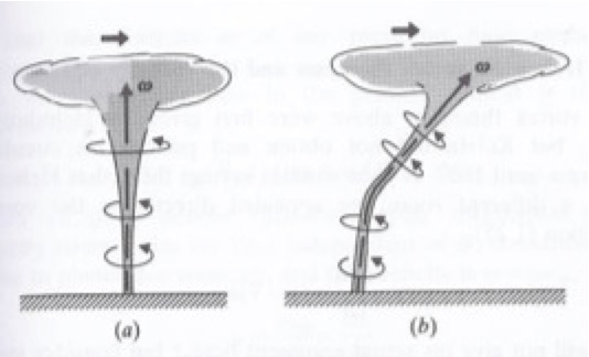
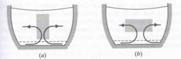
This completes the proof of the first vortex theorem: vortex lines evolve with the fluid. We sometimes say that the vortex lines are `frozen’ in the fluid, meaning that the evolve in the same way as a dye `frozen’ into the fluid would.
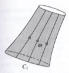
Proof of the second vortex theorem. Proof that \(\Gamma\) is the same for all cross-sections. To prove the second vortex theorem, choose two different cross-sections of the vortex tube, \(S_1\) and \(S_2\) say, and consider the section \(V\) of the vortex tube lying between \(S_1\) and \(S_2\text{.}\) We integrate over the surface of \(V\text{:}\)
\begin{equation*} \iint_{\partial V}\bomega\cdot\bn\de S =\iint_{S_2}\bomega\cdot\bn\de S -\iint_{S_1}\bomega\cdot\bn\de S +\iint_{\mathrm{outside}}\bomega\cdot\bn\de S, \end{equation*}
where `outside’ refers to the outer surface of the vortex tube between \(S_1\) and \(S_2\text{.}\) Since vortex lines are paralled to this surface, we have \(\bomega\cdot\bn=0\) there, and so
\begin{equation*} \iint_{\partial V}\bomega\cdot\bn\de S =\iint_{S_2}\bomega\cdot\bn\de S -\iint_{S_1}\bomega\cdot\bn\de S. \end{equation*}
Now, by the divergence theorem,
\begin{equation*} \iint_{\partial V}\bomega\cdot\bn\de S =\iiint_V\nabla\cdot\omega \de V, \end{equation*}
but this equals zero, since \(\nabla\cdot\omega=0\) (divergence of a curl is zero).
Putting this together,
\begin{equation*} \iint_{\partial V}\bomega\cdot\bn\de S =\iint_{S_2}\bomega\cdot\bn\de S -\iint_{S_1}\bomega\cdot\bn\de S =0. \end{equation*}
and this was true for any choice of \(S_1\) and \(S_2\text{.}\) Hence, \(\Gamma\) is the same for all cross-sections of a vortex tube.
Proof of the second vortex theorem (continued). Proof that \(\Gamma\) is independent of time. To prove that \(\Gamma\) is independent of time, we note that, since the vortex lines move with the fluid, the vortex tube also moves with the fluid, being composed of vortex lines, and the same vortex lines lie on the surface and are enclosed within the vortex tube for all time.
Moreover,
\begin{equation*} \Gamma=\iint\omega\cdot\bn\de S =\oint\bu\cdot\de\bx \end{equation*}
by Stokes’ theorem, which is the circulation around the boundary of \(S\text{.}\) As the tube evolves, the material surface \(S\) moves with the vortex tube. By Kelvin’s circulation theorem Theorem 6.1.2, \(\Gamma\) remains independent of \(t\text{.}\)

Remark 6.2.4.

The second theorem shows us that if a vortex tube becomes stretched then by mass conservation, it must get thinner. The flux of vorticity along the vortex tube is given by \(\Gamma=\int_S\bomega\cdot{\bn}\,dS\text{,}\) and this must remain constant, and therefore, since the area of the cross-section \(S\) is decreasing, the magnitude of vorticiy \(\bomega\) must increase in the tube. This is spin up. Conversely, if a vortex tube becomes shorter, we get the opposite effect of spin down and \(\bomega\) gets smaller.
A non-fluids example of the same principle can be seen when dancers perform moves involving spins, especially ice skaters, the dance starts rotating with their arms or legs out, and then they pull in to speed up the spin.

Example 6.2.5. Everyday examples of spin up and spin down.

Spin up
Figure 6.2.6. Spin up of vorticity as thunderclouds move overhead.
Spin up
Figure 6.2.7. Spin down of a cup of tea. Secondary circulations (shown by the arrows) tend to spread the material lines out radially. Thus the tall thin column of fluid (a) becomes a short fat one(b).
The two sketches in Figure 6.2.6 and Figure 6.2.7 (taken from [4]) show examples of spin up and spin down, respectively. Spin up occurs in thunderstorms; as the cloud moves, the vortex lines get stretched, and this can result in a tornado. Spin up happens in a cup of tea after it has been stirred. Secondary flows in the cup tend to spread the column of rotating fluid horizontally, making the area of the cross-section of the vortex tube bigger, and hence the vorticity smaller, which is spin down.
There is a nice video of a tornado on Instagram. Due to the fast flow in the tornado, the pressure in the core is very low (this is an application of Bernoulli’s equation), and water condenses out of the air, making the tornado visible.

Example 6.2.8. Plug hole vortex.

We saw the vortex that forms around a plug hole in the movie `Vorticity, Part 1’ at this website.
The presenter commented that the angular momentum of a fluid parcel remains constant. Using angular momentum equals velocity times distance from axis, this implies the angular velocity is proportial to the inverse of the radial distance. This is precisely the
In it, we saw a reference to `Crocco’s theorem’, which can be derived from the derivation of Bernoulli’s equation (3.5.6):
\begin{equation*} \pd{\bu}{t} + \bomega \times \bu = -\nabla B, \end{equation*}
where
\begin{equation*} B = \frac{p}{\rho} + \frac{1}{2} |\bu|^2 + \chi, \end{equation*}
with
\begin{equation*} \bg = -\nabla \chi. \end{equation*}
Noting that this flow is steady and has zero vorticity away from the plughole, we must have \(\bnabla B=0\text{,}\) that is \(B\) is constant everywhere. On the surface, we have \(p=p_{\mathrm{atm}}\) and hence \(|\bu|^2/2 + gz\) is constant, where \(z\) is vertical height. Using (4.2.9), the speed is \(\Gamma/(2\pi r)\text{.}\) Hence, the quantity
\begin{equation*} \frac{\Gamma^2}{8\pi^2r^2}+gz \end{equation*}
is constant, that is
\begin{equation*} z=z_0-\frac{\Gamma^2}{8\pi^2gr^2}, \end{equation*}
thus explaining the shape of the surface that was seen.

Example 6.2.9. Tornado.

As commented in the `Vorticity, Part 2’ at this website, the pressure in the middle of a tornado is very low. This can also be understood from Bernoulli’s equation (3.5.6):
\begin{equation*} \pd{\bu}{t} + \bomega \times \bu = -\nabla B, \end{equation*}
with
\begin{equation*} B = \frac{p}{\rho} + \frac{1}{2} |\bu|^2 + \chi. \end{equation*}
In the steady case, and outside the vortex core, there is no vorticity and hence \(B\) is constant, meaning that, as we approach the vortex core, the pressure decreases as the fluid speed increases. Furthermore, in the vortex core where the vorticity is non-zero, the quantity \(\bomega \times \bu\) points towards the axis. Thus \(B\) decreases as the axis is approached, further decreasing the pressure.
This pressure reduction leads to condensation in the core of the tornado, and this is visible, allowing us to see the tornado, and, to some extent, visualise the intense air flows associated with it.
As commented, in propellors of boats, this pressure reduction in the core of a vortex can cause the water to boil!

Subsection 6.2.2 The Helmholtz principle

Remark 6.2.10. Recap of line vortex.

The Helmholtz vertex theorems help us to understand the concept of a line vortex in irrotational flow that was introduced in Example 4.2.10. Recall that this is associated with the complex potential
\begin{equation*} f(z) = -\frac{\im \Gamma}{2\pi} \log z. \end{equation*}
(see (4.3.7)), and has corresponding velocity components
\begin{equation*} u = -\frac{\Gamma y}{2\pi(x^2+y^2)},\quad v = \frac{\Gamma x}{2\pi(x^2+y^2)}. \end{equation*}
The vorticity associated with this flow \(\bomega=\bzero\) at all points except the singularity at the origin. However, it was also notes in (4.2.10) that the circulation around any closed curve containing the origin is \(\Gamma\text{.}\)
Thus, a line vortex of strength \(\Gamma\) is the limit of a vortex tube of strength \(\Gamma\) as its thickness goes to zero.
We note that in any real fluid, the effects of viscosity would come into play in the core of the line vortex, disallowing an infinite concentration of vorticity there. Despite this, we can use the concept of a line vortex to gain insight into a number of real-world problems.
The following corollary is a useful application of the Helmholtz vortex theorems.

Proof.

A flow with a line vortex has an infinite concentration of vortex lines along the axis of the line vortex. By the first vortex theorem Theorem 6.2.2, these are frozen in the fluid, and thus evolve with the background flow with the line vortex removed.

Remark 6.2.12. Application of the Helmholtz principle.

In the case of a two-dimensional flow containing a line vortex that is everywhere irrotational (apart from in the line vortex core), we can use the Helmholtz principle to find the motion of the line vortex. In particular, to find the evolution of the flow we can make use of the following techniques that were covered in Chapter 4:

Example 6.2.13. Vortex pair.

We assume two-dimensional flow, and consider the evolution of two line vortices of equal and opposite strengths initially a distance \(2d\) apart at locations \((x,y)=(\pm d,0\) with the vortex at \((d,0)\) having strength \(\Gamma\) and that at \((-d,0)\) having strength \(-\Gamma\text{.}\)
The vortex at \((d,0)\) will move under the influence of that at \((-d,0)\) with speed \(\Gamma/(4\pi d)\) in the \(-y\)-direction. Similarly, the vortex \((-d,0)\) will also move with speed \(\Gamma/(4\pi d)\) in the \(-y\)-direction. Since their separation remains constant, the two vortices will continue to move at a constant speed \(\Gamma/(4\pi d)\) in the \(-y\)-direction.
In the frame of reference moving with the vortices, there is a uniform flow \(\Gamma/(4\pi d)\) in the \(+y\)-direction and the flow due to each of the vortices. The complex potential is the sum of the complex potentials due to these three elements:
\begin{equation*} f=-\frac{\im \Gamma z}{4\pi d} -\frac{\im \Gamma}{2\pi}\log\left(z-d\right) +\frac{\im \Gamma}{2\pi}\log\left(z+d\right). \end{equation*}
The streamfunction is the imaginary part of this:
\begin{align*} \psi=&-\frac{\Gamma x}{4\pi d} -\frac{\Gamma}{2\pi}\log\left|z-d\right| +\frac{\Gamma}{2\pi}\log\left|z+d\right|\\ =&-\frac{\Gamma}{4\pi}\left(\frac{x}{d}+2\log\left|\frac{z-d}{z+d}\right|\right)\\ =&-\frac{\Gamma}{4\pi}\left(\frac{x}{d}+\log\left(\frac{(x-d)^2+y^2}{(x+d)^2+y^2}\right)\right). \end{align*}
To help with plotting the streamfunction, we note that:
  • The derivative of the complex potential is
    \begin{equation*} f'=-\frac{\im\Gamma}{4\pi}\left(\frac1d+\frac{2}{z-d}-\frac{2}{z+d}\right), \end{equation*}
    which equals zero at the points \(z=\pm\sqrt{3}\im d\text{,}\) so these are stagnation points of the flow.
  • We have \(\psi=0\) on the line \(x=0\text{,}\) so this is a streamline.
  • Far from the vortices (in any direction), the streamfunction is approximately \(\psi\sim-\Gamma x/(4\pi d)\text{,}\) so the streamlines are approximately vertical lines.
  • As we approach the vortex at \(z=d\text{,}\) \(\psi\) tends to \(-\infty\) and as we approach the vortex at \(z=-d\text{,}\) \(\psi\) tends to \(+\infty\text{.}\)
These points imply that there is a curve on which \(\psi=0\) in the right-half plane. This curve joins the two stagnation points and goes around the vortex. Similarly, there is a curve on which \(\psi=0\) in the left-half plane, and these two curves are reflections of one another.
If we dye the fluid within these two curves, we would create a blob of fluid surrounding the vortices. An observer would see this blob of fluid travelling at the speed \(\Gamma/(4\pi d)\) in the \(-y\)-direction without changing shape, see Figure Figure 6.2.14b.
Vortex pair
Figure 6.2.14. Flow due to a vortex pair relative to (a) a fixed frame, and (b) a frame moving with the vortices. Note that the shaded region in (b) represents a fluid region that, if it were dyed, the dyed fluid would remain in the same region throughout the evolution of the flow. From [4].

Example 6.2.15. Vortex near a wall.

Consider a vortex of strength \(\Gamma\) at a distance \(d\) from a flat wall.
Solution.
This can be analysed using the method of images, and we put an image vortex a distance \(d\) on the other side of the wall, directly opposite the real vortex, also of strength \(-\Gamma\text{.}\) Then the problem is equivalent to that of two vortices in free space, and we can use the result from the previous example to find the motion of the vortex.

Example 6.2.16. Example: Wing tip vortices.

(From Exercise 5.8 in [4]). An inviscid fluid occupies the region \(x,y\geq0\text{,}\) and is bounded by rigid boundaries at \(x=0\) and at \(y=0\text{.}\) Its motion results wholly from the presence of a line vortex of strength \(\Gamma\text{.}\) Show that the path taken by the vortex is
\begin{equation*} \frac1{x^2}+\frac1{y^2}=\mathrm{constant}. \end{equation*}
At take-off, an aircraft generates strong vortices shed from the tips of its wings, see Figure 6.0.2. These are observed to move downwards and outwards under each other’s influence.
Solution.
Suppose the vortex is at the point
\begin{equation*} z_1=x_1+\im y_1. \end{equation*}
We use three image vortices at \(x_1-\im y_1\) and at \(-x_1+\im y_1\text{,}\) both of strength \(-\Gamma\text{,}\) and at \(-x_1-\im y_1\) of strength \(\Gamma\text{.}\)
Recall that the complex potential of a line vortex at \(z=c\) of strength \(\Gamma\) is \(-\im\Gamma\log(z-c)/(2\pi)\) and its velocity is given by the derivative of this map: \(u-\im v=-\im\Gamma/(2\pi(z-c))\text{.}\)
The velocity of the vortex is given by the sum of the velocities due to the other three vortices:
\begin{align*} \dd{x_1}{t}-\im\dd{y_1}{t} =&\frac{\im\Gamma}{2\pi((x_1+\im y_1)-(x_1-\im y_1))}\\ &+\frac{\im\Gamma}{2\pi((x_1+\im y_1)-(-x_1+\im y_1))}\\ &-\frac{\im\Gamma}{2\pi((x_1+\im y_1)-(-x_1-\im y_1))}\\ &=\frac{\im\Gamma}{4\pi}\left(\frac1{x_1}+\frac1{\im y_1}-\frac1{x_1+\im y_1}\right). \end{align*}
Hence
\begin{gather*} \dd{x_1}{t} =\frac{\Gamma}{4\pi}\left(\frac1{y_1}-\frac{y_1}{x_1^2+y_1^2}\right) =\frac{\Gamma x_1^2}{4\pi y_1(x_1^2+y_1^2)},\\ \dd{y_1}{t} =\frac{\Gamma}{4\pi}\left(-\frac1{x_1}+\frac{x_1}{x_1^2+y_1^2}\right) =-\frac{\Gamma y_1^2}{4\pi x_1(x_1^2+y_1^2)}, \end{gather*}
and therefore
\begin{equation*} \dd{y_1}{x_1}=-\frac{y_1^3}{x_1^3}, \end{equation*}
which can be solved by separation of variables to give
\begin{equation*} \int\frac1{y_1^3}\de y_1=-\int\frac1{x_1^3}\de x_1 \quad\Rightarrow\quad -\frac1{2y_1^2}=\frac1{2x_1^2}+c, \end{equation*}
where \(c\) is constant, and this can be rearranged into the required form.

Example 6.2.17. Application to airports.

At a busy airport, a delay is required between the take off of one aircraft and the next in order for the wing tip vortices generated from the take off of the first aircraft to move away and break up. The time required for this to happen depends on the size and speed of the aircraft, as well as the angle of attack of the wings, but it is typically 2 or 3 minutes. This need for a delay is the main reason that a given airport runway can only take so many aeroplanes per day, limiting the flight volume of the airport.
You will have heard recent debate about the controversy surrounding the building of a third runway at London Heathrow, the busiest airport in the UK. Although not explained by the media coverage, you now understand the crucial role played by the fluid dynamics that underlies these arguments!