Stress in a fluid

Section 7.3 Stress in a fluid

Subsection 7.3.1 Stress at a surface

Definition 7.3.1. Definition of stress at a surface.

The fluid stress on a surface, \(\btau\text{,}\) is the force per unit area exerted by the fluid; note that this is a vector quantity. It is often convenient to decompose the stress into two contributions, as these are often quite different both in magnitude and in physical origin:

Shear stress: the components tangential to the surface

🔗
Normal stress: the component perpendicular to the surface.

🔗

🔗

Example 7.3.2. Fluid stress in arteries.

The shear stress on arterial walls is everywhere maintained at around \(\sim1.5\) Pa, whereas the normal stress is typically much larger at ~11–16 kPa. The distribution of shear stress, although much smaller than the normal stress, is known to be of great importance to our health as it is linked to the development of atherosclerosis, which leads to heart attacks and strokes, two of the leading causes of death worldwide.

🔗

Definition 7.3.3. Calculation of stress at a surface.

For Newtonian fluids at a no-slip surface:

The wall shear stress equals the fluid shear viscosity multiplied by the normal derivative of the tangential velocity.

🔗
Provided the surface is not accelerating, the normal stress equals the pressure.

🔗

Note that in 3D there are two shear components and one normal component.

🔗

Example 7.3.4. Shear stress at a flat wall.

Flat wall at \(z=0\) and fluid in \(z>0\text{:}\)

\begin{equation*} \tau_x = \mu\pd{u}{z},\quad \tau_y = \mu\pd{v}{z}. \end{equation*}

Flat wall at \(z=0\) and fluid in \(z<0\text{:}\)

\begin{equation*} \tau_x = -\mu\pd{u}{z},\quad \tau_y = -\mu\pd{v}{z}. \end{equation*}

🔗

Example 7.3.5. Shear stress on a circular pipe.

Flow in a circular pipe, wall at \(r=a\) in cylindrical polar coordinates:

\begin{equation*} \tau_{\textrm{axial}} = -\mu\pd{u_z}{r},\quad \tau_{\textrm{azimuthal}} = -\mu\pd{u_{\theta}}{r}. \end{equation*}

🔗

Example 7.3.6. Cone-and-plate viscometer.

Cone-and-plate viscometer: cone lowered into fluid, torque needed to rotate cone gives viscosity.

🔗

Example 7.3.8. Falling ball viscometer.

Falling-ball viscometer: measure terminal velocity of a ball in fluid at low Reynolds number (see Figure 7.0.2).

🔗

Subsection 7.3.2 The stress tensor

Cauchy showed that the state of stress at a point in a continuum body is completely defined by a rank two tensor (that is, a matrix with appropriate transformation properties) called the Cauchy stress tensor, \(\bsigma(\bx,t)\text{,}\) given by

\begin{equation} \bsigma=\left(\begin{matrix} \sigma_{11} & \sigma_{12} & \sigma_{13} \\ \sigma_{21} & \sigma_{22} & \sigma_{23} \\ \sigma_{31} & \sigma_{32} & \sigma_{33} \end{matrix}\right),\tag{7.3.1} \end{equation}

which has nine scalar components.

🔗

Definition 7.3.9. Obtaining the stress from the stress tensor.

Definition 7.3.1 can be extended to any surface within the fluid. The stress is a vector (or rank one tensor), \(\btau\text{,}\) given by

\begin{equation} \btau(\bn)=\bsigma\bn,\tag{7.3.2} \end{equation}

where \(\bn\) is the unit normal vector to the surface, pointing into the fluid that is giving rise to the stress.

🔗

Remark 7.3.10. Element interpretation of the stress tensor.

The element \(\sigma_{ij}\) of the stress tensor can be defined as the \(i\)th component of the stress on the plane with normal vector \(\be_j\) in the direction of increasing \(x_j\text{.}\)

🔗

Thus for example \(\sigma_{23}(x,y,z_0,t)\) is the \(y\)-component of the stress on the surface \(z=z_0\) within the fluid, and acting on the fluid in \(z>z_0\text{.}\) There is an equal and opposite stress acting on the fluid in \(z<z_0\text{.}\)

🔗

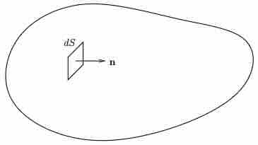
Remark 7.3.11. Notes about the stress tensor.

The stress \(\btau\) is the force per unit area exerted by the fluid on the right-hand side of the small imaginary surface \(dS\) shown in the figure below upon the fluid on the left-hand side of \(dS\text{.}\)
🔗

Figure 7.3.12. Imaginary surface in a flowing fluid, illustrating the concept of stress within a fluid.
🔗
🔗
The stresses acting on opposite sides of a surface (i.e. on the surfaces with normals \(\bn\) and \(-\bn\)) are equal and opposite. This is required for linear equilibrium within the fluid.
🔗

🔗
The stress tensor is symmetric, i.e. \(\sigma_{ij}=\sigma_{ji}\text{.}\) This is required for rotational equilibrium within the fluid, and can be derived from the principle of conservation of angular momentum.
🔗

🔗
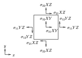
The elements on the principal diagonal of the stress tensor matrix are called the normal stresses. The other six elements are called the shear stresses. The diagram below illustrates this; a cuboid with side lengths \(X\text{,}\) \(Y\) and \(Z\) in the \(x\)-, \(y\)- and \(z\)-directions, respectively, is shown, and the \(x\)- and \(y\)-components of the stresses on those faces that can be seen are shown.
🔗

Figure 7.3.13. Components of the stress on the faces of a small cuboid within a fluid.
🔗
In Figure 7.3.13:
- The \(z\)-components of the stresses are not shown in order that the diagram does not get too complicated (also the stress on the back face is not shown).
  🔗
  
  🔗
- The \(z\)-axis points outwards from the figure – right-handed axes.
  🔗
  
  🔗
- Note that these forces assume that the components of the stress tensor are uniform over the faces in question, which would not generally be the case, (although it is quite accurate in the case that the lengths \(X\text{,}\) \(Y\) and \(Z\) are small.
  🔗
  
  🔗
🔗
🔗

🔗

Remark 7.3.14. Defining the fluid pressure in terms of the stress tensor.

We can now write a mathematical definition of the fluid pressure in terms of the stress tensor:

\begin{equation} p=-\frac13\textrm{tr}\left(\bsigma\right)=-\frac13\textrm{tr}\left(\bsigma\right).\tag{7.3.3} \end{equation}

This equation gives us a method by which we can (at least in our imagination) think about measuring the pressure at a particular point in the fluid. We consider three small, mutually orthogonal planes passing through the point (aligned perpendicular to the \(x\)-, \(y\)- and \(z\)-directions) and measure the three forces on the three surfaces. Dividing each force by the area of the respective plane leads to the stresses on the surfaces, which are, respectively,

\begin{equation*} \left(\begin{matrix}\sigma_{11}\\\sigma_{21}\\\sigma_{31}\end{matrix}\right),\quad \left(\begin{matrix}\sigma_{12}\\\sigma_{22}\\\sigma_{32}\end{matrix}\right), \quad\textrm{and}\quad \left(\begin{matrix}\sigma_{13}\\\sigma_{23}\\\sigma_{33}\end{matrix}\right). \end{equation*}

The normal components of the respective stresses are \(\sigma_{11}\text{,}\) \(\sigma_{22}\) and \(\sigma_{33}\text{,}\) and hence the pressure is the average of the three normal components of the stresses. The interpretation of the pressure is different for compressible and incompressible fluids:

Compressible fluids: From classical thermodynamics it is known that we can define the pressure of the fluid as a parameter of state, making use of an equation of state (for example \(p=\rho RT\) for an ideal gas).
🔗

🔗
Incompressible fluids: For an incompressible fluid the pressure \(p\) is an independent, purely dynamical, variable.
🔗

🔗

In this course we mainly consider incompressible fluids.

🔗

Remark 7.3.15. Notes about the stress tensor and pressure.

(7.3.3) naturally leads to

\begin{equation*} \sigma_{ij}=-p \delta_{ij}+d_{ij}, \end{equation*}

where \(\bd=(d_{ij})\) is called the deviatoric stress tensor, and this part of the stress occurs entirely due to the fluid motion. Taking the trace of this equation gives \(\textrm{tr}(\bsigma)=-3p+\textrm{tr}(\bd)\text{,}\) and (7.3.3) implies that \(\textrm{tr}(\bd)=\boldsymbol{0}\text{.}\)

🔗

Remark 7.3.16. Special case of a fluid at rest.

In a fluid at rest we have \(d_{ij}=0\text{,}\) and thus \(\bsigma=-p\bI\text{,}\) where \(\bI\) is the identity matrix, meaning that \(\bsigma\) is a multiple of the identity matrix and the only stresses are due to the pressure.

🔗

Definition 7.3.17. The constitutive relationship of a fluid.

This is an equation that describes the relationship between the stress tensor and the kinematic state of the fluid. It is found from experiments, and governs the mechanical behaviour of the fluid, that is the rheology of the fluid. Together with the equations of mass and momentum conservation, this closes the problem for the velocity and pressure fields. Every fluid obeying the continuum approximation has a constitutive relationship, which can be thought of as a definition of its mechanical properties.

🔗

Prev Top Next