Conservation of linear momentum

Section 7.5 Conservation of linear momentum

We consider the balance of linear momentum in a small cube of side length \(\delta\) for an incompressible fluid, see Figure 7.5.1. To do this we employ the Reynolds Transport Theorem (3.1.2), with \(\bf(\bx,t)\) equal to the linear momentum of the fluid per unit volume, \(\bf=\rho\bu\text{,}\) and \(V(t)\) being the small volume of fluid under consideration, which coincides with the cube at time \(t\) (however, note that the volume of fluid we are following is not generally a cube at other times). Substituting \(\bf=\rho\bu\text{,}\) the theorem states that:

\begin{equation*} \dd{}{t} \iiint_{V(t)} \rho\bu \, \de{x} \, \de{y} \, \de{z} = \iiint_{V(t)} \left[ \pd{\rho\bu}{t} + \nabla \cdot (\rho\bu\otimes\bu)\right] \, \de{x} \, \de{y} \, \de{z}. \end{equation*}

🔗

Subsection 7.5.1 Left-hand side

We note that \(\iiint_{V(t)} \rho\bu \, \de{x} \, \de{y} \, \de{z}\) is the integral of the linear momentum per unit volume over the volume and is therefore the total momentum of the fluid particles in \(V(t)\text{.}\) The left-hand side of this equation is thus the Lagrangian rate of change of momentum of these fluid particles. By Newton’s second law, this must equal the resultant force acting on the fluid in \(V(t)\text{,}\) which we denote by \(\bF\text{.}\) This force is the sum of different contributions, which can be categorised into body forces (which act on the whole volume of fluid) and surface forces (acting only on the surface of the fluid, and which arise from the fluid stress):

\begin{equation*} \dd{}{t} \iiint_{V(t)} \rho\bu \, \de{x} \, \de{y} \, \de{z} = \bF = \bF_{\textrm{body}} + \bF_{\textrm{surface}}. \end{equation*}

🔗

Body forces: In this course, these are equal to either zero (if gravity is not important) or equal to the gravitational force

\begin{equation*} \bF_{\textrm{surface}}=\bF_{\textrm{gravity}}=\rho V\bg. \end{equation*}

🔗

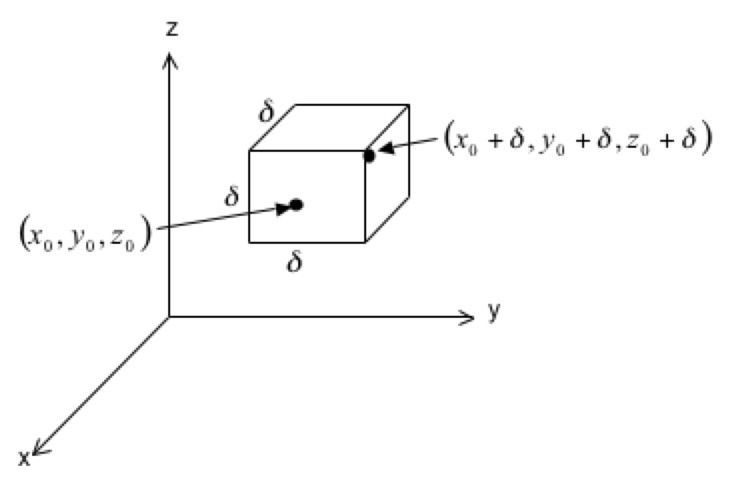
Surface forces: These arise from the stress exerted at the surface of the fluid parcel, and these can be computed by integrating the stress vector \(\tau\) over the surface of the cube. On the left face, we have \(\bn=-\bi\text{,}\) and, using (7.4.5), the stress vector is

\begin{align*} \btau=&\bsigma\bn\\ =&\left(-p\bI+2\mu\be\right)\left(-\bi\right)\\ =&\left(\begin{matrix} -p+2\mu\pd{u}{x}&\mu\left(\pd{u}{y}+\pd{v}{x}\right)&\mu\left(\pd{u}{z}+\pd{w}{x}\right)\\ \mu\left(\pd{u}{y}+\pd{v}{x}\right)&-p+2\mu\pd{v}{y}&\mu\left(\pd{v}{z}+\pd{w}{y}\right)\\ \mu\left(\pd{u}{z}+\pd{w}{x}\right)&\mu\left(\pd{v}{z}+\pd{w}{y}\right)&-p+2\mu\pd{w}{z} \end{matrix}\right) \left(\begin{matrix}-1\\0\\0\end{matrix}\right)\\ =&-\left(\begin{matrix} -p+2\mu\pd{u}{x}\\ \mu\left(\pd{u}{y}+\pd{v}{x}\right)\\ \mu\left(\pd{u}{z}+\pd{w}{x}\right) \end{matrix}\right), \end{align*}

and the force on the left face is this expression multiplied by the area \(\delta^2\text{.}\) Similarly, on the right-hand face, we have \(\bn=\bi\text{,}\) and the stress vector is

\begin{equation*} \btau=\bsigma\bn =\left(\begin{matrix} -p+2\mu\pd{u}{x}\\ \mu\left(\pd{u}{y}+\pd{v}{x}\right)\\ \mu\left(\pd{u}{z}+\pd{w}{x}\right) \end{matrix}\right), \end{equation*}

with the contribution to the force being this expression multiplied by \(\delta^2\text{.}\) Hence the contribution to the force from the left and right faces is

\begin{align*} &\left.\left(\begin{matrix} -p+2\mu\pd{u}{x}\\ \mu\left(\pd{u}{y}+\pd{v}{x}\right)\\ \mu\left(\pd{u}{z}+\pd{w}{x}\right) \end{matrix}\right)\delta^2\right|_{x=x_0+\delta} -\left.\left(\begin{matrix} -p+2\mu\pd{u}{x}\\ \mu\left(\pd{u}{y}+\pd{v}{x}\right)\\ \mu\left(\pd{u}{z}+\pd{w}{x}\right) \end{matrix}\right)\delta^2\right|_{x=x_0}\\ =&\pd{}{x}\left(\begin{matrix} -p+2\mu\pd{u}{x}\\ \mu\left(\pd{u}{y}+\pd{v}{x}\right)\\ \mu\left(\pd{u}{z}+\pd{w}{x}\right) \end{matrix}\right)\delta^3\\ =&\pd{}{x}\left(\begin{matrix} -p+2\mu\pd{u}{x}\\ \mu\left(\pd{u}{y}+\pd{v}{x}\right)\\ \mu\left(\pd{u}{z}+\pd{w}{x}\right) \end{matrix}\right)V. \end{align*}

After a similar calculation, the contributions from the front and back faces can be shown to be

\begin{equation*} \pd{}{y}\left(\begin{matrix} \mu\left(\pd{v}{x}+\pd{u}{y}\right)\\ -p+2\mu\pd{v}{y}\\ \mu\left(\pd{v}{z}+\pd{w}{y}\right) \end{matrix}\right)V, \end{equation*}

and from the top and bottom faces we get

\begin{equation*} \pd{}{z}\left(\begin{matrix} \mu\left(\pd{w}{x}+\pd{u}{z}\right)\\ \mu\left(\pd{w}{y}+\pd{v}{z}\right)\\ -p+2\mu\pd{w}{z} \end{matrix}\right)V. \end{equation*}

Hence the total force due to surface stresses is

\begin{align*} \bF_{\textrm{surface}}=\bF_{\textrm{stress}}=& \pd{}{x}\left(\begin{matrix} -p+2\mu\pd{u}{x}\\ \mu\left(\pd{u}{y}+\pd{v}{x}\right)\\ \mu\left(\pd{u}{z}+\pd{w}{x}\right) \end{matrix}\right)V +\pd{}{y}\left(\begin{matrix} \mu\left(\pd{v}{x}+\pd{u}{y}\right)\\ -p+2\mu\pd{v}{y}\\ \mu\left(\pd{v}{z}+\pd{w}{y}\right) \end{matrix}\right)V +\pd{}{z}\left(\begin{matrix} \mu\left(\pd{w}{x}+\pd{u}{z}\right)\\ \mu\left(\pd{w}{y}+\pd{v}{z}\right)\\ -p+2\mu\pd{w}{z} \end{matrix}\right)V\\ =& \left(\begin{matrix} -\pd{p}{x}+\mu\left(\pd{^2u}{x^2}+\pd{^2v}{x\partial y}+\pd{^2w}{x\partial z}+\nabla^2u\right)\\ -\pd{p}{y}+\mu\left(\pd{^2u}{x\partial y}+\pd{^2v}{y^2}+\pd{^2w}{y\partial z}+\nabla^2v\right)\\ -\pd{p}{z}+\mu\left(\pd{^2u}{x\partial z}+\pd{^2v}{y\partial z}+\pd{^2w}{z^2}+\nabla^2w\right) \end{matrix}\right)V\\ =&\left(-\nabla p+\mu\left(\nabla\pd{u}{x}+\nabla\pd{v}{y}+\nabla\pd{w}{z}\right) +\mu\nabla^2\bu\right)V\\ =&\left(-\nabla p+\mu\nabla\nabla\cdot\bu+\mu\nabla^2\bu\right)V\\ =&\left(-\nabla p+\mu\nabla^2\bu\right)V, \end{align*}

where the final equality was obtained using the incompressibility condition \(\nabla\cdot\bu=0\) (3.4.2).

🔗

Hence, the left-hand side of the Reynolds Transport Theorem becomes

\begin{equation*} \dd{}{t} \iiint_{V(t)} \rho\bu \, \de{x} \, \de{y} \, \de{z} = \bF_{\textrm{body}} + \bF_{\textrm{surface}} = \left(\rho\bg-\nabla p + \mu\nabla^2\bu\right)V. \end{equation*}

🔗

Subsection 7.5.2 Right-hand side

We now evaluate the right-hand side of the Reynolds Transport Theorem:

\begin{align*} & \iiint_{V(t)} \left[ \pd{(\rho\bu)}{t} + \nabla \cdot (\rho\bu\otimes\bu)\right] \, \de{x} \, \de{y} \, \de{z}\\ =& \iiint_{V(t)} \rho\left[ \pd{\bu}{t} + (\bu\cdot\nabla)\bu+\bu(\nabla\cdot\bu)\right] \, \de{x} \, \de{y} \, \de{z}\\ =& \iiint_{V(t)} \rho\left[ \pd{\bu}{t} + (\bu\cdot\nabla)\bu\right] \, \de{x} \, \de{y} \, \de{z}, \end{align*}

where the final equality was obtained using the incompressibility condition \(\nabla\cdot\bu=0\) (3.4.2).

🔗

Subsection 7.5.3 Equating the two sides

Setting the two sides equal gives

\begin{equation*} \left(\rho\bg-\nabla p + \mu\nabla^2\bu\right)V=\iiint_{V(t)} \rho\left[ \pd{\bu}{t} + (\bu\cdot\nabla)\bu\right] \, \de{x} \, \de{y} \, \de{z}, \end{equation*}

and since this must hold for any small volume of fluid, we obtain

\begin{equation*} \rho\bg-\nabla p + \mu\nabla^2\bu=\rho\left[ \pd{\bu}{t} + (\bu\cdot\nabla)\bu\right]. \end{equation*}

Rearranging gives the incompressible Navier–Stokes equation:

\begin{equation} \boxed{\rho\DD{\bu}{t} =-\nabla p+\mu\nabla^2\bu+\rho{\bg}.}\tag{7.5.1} \end{equation}

🔗

Remark 7.5.2. Clarification on the detail of the proof.

Note that there was some sleight of hand going on in this proof! We assumed that the stress was uniform over each face of the cube, meaning we could just multiply the stress on each face by the area of the face to get the force on that face. Indeed, if this were actually the case, then the stress would be uniform over the whole surface of the cube, and hence the net force on the surface would be zero. To resolve this, we would need to add higher-order contributions into the integrand when calculating the force on each face, which could result in higher-order contributions to the resultant force due to the sum of the stresses. We could do this by writing the stress as a Taylor series about the corner of the cube. Happily, with a bit more work (not included here), these higher order terms cancel and the result we obtained here holds.

🔗

Remark 7.5.3.

The incompressible Navier–Stokes equation (7.5.1) together with the incompressible continuity equation (3.4.2) is often used to study problems encountered in fluid dynamics and it was developed by Claude-Louis Navier (1785–1836) and George Gabriel Stokes (1819–1903).

🔗

Subsection 7.5.4 Discussion of the Navier–Stokes equation

Remark 7.5.4. Inertial terms.

The terms on the left-hand side of (7.5.1) represent inertial effects, since the material derivative

\begin{equation*} \DD{\bu}{t}=\pd{\bu}{t}+(\bu\cdot\nabla)\bu \end{equation*}

is the acceleration moving with the fluid. Thus the left-hand side is rate of change of momentum of the fluid particles per unit volume of the fluid. As remarked earlier in this course, it is not surprising that the material derivative appears in the governing equations, since forces act on fluid particles.

🔗

Remark 7.5.5. Solving the equations.

The Navier–Stokes equation is notoriously difficult to solve, particularly as the term

\begin{equation*} \rho\bu\cdot\nabla\bu \end{equation*}

is nonlinear. In fact, one of the famous Millennium Prize Problems is to prove that in three dimensions, given suitable initial and boundary conditions, there always exists a smooth solution of the Navier–Stokes equation for all time, or to provide an example where this does not hold. The problem is that the nonlinear term can lead to singularities developing in the solution, which would correspond to infinite velocities or pressures at some point in the fluid. This is not expected to happen in real fluids, but proving this rigorously is a major challenge.

🔗

You will be relieved to know that in this course we will only consider simple solutions of the Navier–Stokes equations (often ones in which the nonlinear term equals zero).

🔗

In a typical problem, there are four unknown variables: \(u\text{,}\) \(v\text{,}\) \(w\) and \(p\text{.}\) There are four equations governing their behaviour, which are the incompressible continuity equation (3.4.2) and the three components of the Navier–Stokes equation (7.5.1). In addition, we need to specify appropriate boundary conditions (for example, no slip conditions at a solid boundary) and initial conditions (the velocity and pressure at time \(t=0\)).

🔗

Remark 7.5.6. Equations in components.

The Navier–Stokes and continuity equations (7.5.1) and (3.4.2) can be written in component form as

\begin{align*} &\rho\left(\pd{u}{t}+u\pd{u}{x}+v\pd{u}{y}+w\pd{u}{z}\right)=-\pd{p}{x}+\mu\left(\pd{^2u}{x^2}+\pd{^2u}{y^2}+\pd{^2u}{z^2}\right)+\rho g_x,\\ &\rho\left(\pd{v}{t}+u\pd{v}{x}+v\pd{v}{y}+w\pd{v}{z}\right)=-\pd{p}{y}+\mu\left(\pd{^2v}{x^2}+\pd{^2v}{y^2}+\pd{^2v}{z^2}\right)+\rho g_y,\\ &\rho\left(\pd{w}{t}+u\pd{w}{x}+v\pd{w}{y}+w\pd{w}{z}\right)=-\pd{p}{z}+\mu\left(\pd{^2w}{x^2}+\pd{^2w}{y^2}+\pd{^2w}{z^2}\right)+\rho g_z,\\ &\pd{u}{x}+\pd{v}{y}+\pd{w}{z}=0. \end{align*}

Or, in two dimensions:

\begin{align*} &\rho\left(\pd{u}{t}+u\pd{u}{x}+v\pd{u}{y}\right)=-\pd{p}{x}+\mu\left(\pd{^2u}{x^2}+\pd{^2u}{y^2}\right)+\rho g_x,\\ &\rho\left(\pd{v}{t}+u\pd{v}{x}+v\pd{v}{y}\right)=-\pd{p}{y}+\mu\left(\pd{^2v}{x^2}+\pd{^2v}{y^2}\right)+\rho g_y,\\ &\pd{u}{x}+\pd{v}{y}=0. \end{align*}

🔗

The special case of an axisymmetric flow (one that is rotationally symmetric) is also much simpler to analyse (and sometimes this is also referred to as being two-dimensional).

🔗

Remark 7.5.7. Comparison with analysis of the extensive properties.

Non-examinable.

🔗

As mentioned in Remark 3.1.7, some engineering problems can be analysed in terms of applying the principle of mass and linear momentum conservation to a defined region of the fluid, and this can be used for some engineering applications. In contrast, the Navier–Stokes and continuity equations, (7.5.1) and (3.4.2), apply mass and linear momentum conservation at each point in the fluid.

🔗

Remark 7.5.8. The Cauchy equation.

Instead of working in terms of the stress tensor for Newtonian fluids, as we did in the derivation of the Navier–Stokes equation (7.5.1), we can instead work in terms of a general stress tensor to derive the Cauchy equation, which applies to any fluid. This states

\begin{equation} \rho\DD{\bu}{t}=\nabla\cdot\bsigma+\rho\bf,\tag{7.5.2} \end{equation}

where \(\bf\) is the body force per unit mass (for example, gravity). This is a more general equation than the Navier–Stokes equation, which applies only to Newtonian fluids obeying the consititutive law (7.4.5). You will perform the derivation in this more general case in Exercise 7.9.10.

🔗

Remark 7.5.9. Non-inertial reference frames.

The Navier–Stokes equations can be adapted for use in a non-inertial reference frame:

\begin{equation*} \rho\left(\pd{\bu_n}{t}+\bu_n\cdot\nabla_n\bu_n\right) =-\nabla_n p+\mu\nabla_n^2\bu_n+\rho\bf_{\textrm{apparent}}+\rho\bg_n, \end{equation*}

where \(\bu_n\) and \(\nabla_n\) are, respectively, the velocity and gradient operator in the non-inertial coordinates, and \(\bf_{\textrm{apparent}}\) is the apparent additional force acting on the fluid due to the non-inertial nature of the reference frame, which has contributions due to the linear acceleration and angular accelerations of the non-inertial reference frame, and the Coriolis and centrifugal forces.

🔗

Remark 7.5.10. Inviscid fluids.

In the case of an inviscid fluid, \(\mu=0\text{,}\) and we recover the Euler equation (3.4.5).

🔗

Remark 7.5.11. Navier–Stokes and continuity equations in cylindrical coordinates.

In cylindrical coordinates \((r,\theta,z)\) the continuity equation is

\begin{equation*} \frac1r\pd{(ru_r)}{r}+\frac1r\pd{u_\theta}{\theta}+\pd{u_z}{z}=0, \end{equation*}

and the Navier–Stokes equations are

\begin{gather*} \rho\left(\pd{u_r}{t}+u_r\pd{u_r}{r}+\frac{u_{\theta}}{r}\pd{u_r}{\theta}+u_z\pd{u_r}{z}-\frac{u_{\theta}^2}{r}\right) =-\pd{p}{r} +\mu\left(\nabla^2u_r-\frac{u_r}{r^2}-\frac{2}{r^2}\pd{u_\theta}{\theta}\right)+\rho f_r,\\ \rho\left(\pd{u_{\theta}}{t}+u_r\pd{u_{\theta}}{r}+\frac{u_{\theta}}{r}\pd{u_{\theta}}{\theta}+u_z\pd{u_{\theta}}{z}+\frac{u_ru_{\theta}}{r}\right) =-\frac{1}{r}\pd{p}{\theta} +\mu\left(\nabla^2u_\theta+\frac{2}{r^2}\pd{u_r}{\theta}-\frac{u_{\theta}}{r^2}\right)+\rho f_{\theta},\\ \rho\left(\pd{u_z}{t}+u_r\pd{u_z}{r}+\frac{u_{\theta}}{r}\pd{u_z}{\theta}+u_z\pd{u_z}{z}\right) =-\pd{p}{z} +\mu\nabla^2u_z+\rho f_z, \end{gather*}

where the Laplacian is defined by its action on a function \(A(r,\theta,z)\text{:}\)

\begin{equation*} \nabla^2A=\frac1r\pd{}{r}\left(r\pd{A}{r}\right)+\frac1{r^2}\pd{^2A}{\theta^2}+\pd{^2A}{z^2}, \end{equation*}

and \(\bf=(f_r,f_\theta,f_z)\) represents the body forces per unit mass acting on the fluid. In the case of gravity we set \(\bf=\rho{\bg}\text{,}\) where \(\bg=(0,0,-g)\) is the acceleration due to gravity.

🔗

Note that the vector calculus operators in cylindrical (and also in spherical) coordinates are quite complicated. I would always recommend looking up the formulae, because they is very tricky to remember and extremely time-consuming to derive. A helpful website that lists these formulae along with many other useful formulae is here, and [4] gives these formulae in the appendices, as do many other textbooks. Note in particular that the Laplacian of a vector quantity is not given by the Laplacians of its components individually.

🔗

Remark 7.5.12. Navier–Stokes and continuity equations in spherical coordinates.

In spherical coordinates \((r,\theta,\phi)\) the continuity equation is

\begin{equation*} \frac1{r^2}\pd{(r^2u_r)}{r}+\frac1{r\sin\theta}\pd{(u_\theta\sin\theta)}{\theta}+\frac1{r\sin\theta}\pd{u_\phi}{\phi}=0, \end{equation*}

and the Navier–Stokes equations are

\begin{gather*} \rho\left(\pd{u_r}{t}+u_r \pd{u_r}{r}+\frac{u_{\theta}}{r}\pd{u_r}{\theta}+\frac{u_{\phi}}{r \sin\theta}\pd{u_r}{\phi}-\frac{u_{\phi}^2+u_{\theta}^2}{r}\right) =-\pd{p}{r} +\mu\left(\nabla^2u_r-\frac{2u_r}{r^2}-\frac2{r^2\sin\theta}\pd{}{\theta}\left(u_\theta\sin\theta\right) +\frac{2}{r^2\sin\theta}\pd{u_{\phi}}{\phi} \right) +\rho f_r,\\ \rho\left(\pd{u_\theta}{t}+u_r\pd{u_{\theta}}{r}+\frac{u_{\theta}}{r}\pd{u_{\theta}}{\theta}+\frac{u_{\phi}}{r\sin\theta}\pd{u_{\theta}}{\phi}+\frac{u_ru_{\theta}-u_{\phi}^2\cot\theta}{r}\right) =-\frac1r\pd{p}{\theta} +\mu\left(\nabla^2u_\theta-\frac{u_\theta}{r^2\sin^2\theta}+\frac2{r^2}\pd{u_r}{\theta}-\frac{2\cos\theta}{r^2\sin^2\theta}\pd{u_\phi}{\phi}\right) +\rho f_\theta,\\ \rho\left(\pd{u_{\phi}}{t}+u_r\pd{u_{\phi}}{r}+\frac{u_{\theta}}{r}\pd{u_{\phi}}{\theta}+\frac{u_{\phi}}{r\sin\theta}\pd{u_{\phi}}{\phi}+\frac{u_ru_{\phi}+u_{\phi}u_{\theta}\cot\theta}{r}\right) =-\frac1{r\sin\theta}\pd{p}{\phi} +\mu\left(\nabla^2u_\phi-\frac{u_\phi}{r^2\sin^2\theta}+\frac{2}{r^2\sin\theta}\pd{u_r}{\phi}+\frac{2\cos\theta}{r^2\sin^2\theta}\pd{u_\theta}{\phi}\right) +\rho f_\phi, \end{gather*}

where the Laplacian is defined by its action on a function \(A(r,\theta,\phi)\text{:}\)

\begin{equation*} \nabla^2A=\frac1{r^2}\pd{}{r}\left(r^2\pd{A}{r}\right)+\frac1{r^2\sin\theta}\pd{}{\theta}\left(\sin\theta\pd{A}{\theta}\right)+\frac1{r^2\sin^2\theta}\pd{^2A}{\phi^2}, \end{equation*}

and \(\bf=(f_r,f_\theta,f_\phi)\) represents the body forces per unit mass acting on the fluid. Again in the case of gravity we set \(\bf=\rho{\bg}\text{,}\) where \(\bg=(-g\cos\theta,g\sin\theta,0)\text{.}\)

🔗

Subsection 7.5.5 Example of the application

Example 7.5.13. Application of Navier–Stokes and continuity equations.

Consider an incompressible Newtonian fluid flowing in a gravitational field \(\bg=-g\bk\) with velocity

\begin{equation*} \bu=Kx\bi+Ky\bj-2Kz\bk. \end{equation*}

Check that this flow satisfies the continuity and Navier–Stokes equations, and find the pressure field. Based on Problem 4.34 in [9].

🔗

Solution.

To check the continuity equation, we show

\begin{equation*} \nabla\cdot\bu=K+K-2K=0, \end{equation*}

so this is satisfied.

🔗

The Navier–Stokes equations are

\begin{equation*} \rho\left(\pd{\bu}{t} +(\bu\cdot\nabla)\bu\right) =-\nabla p+\mu\nabla^2\bu-\rho g\bk. \end{equation*}

For the flow given

\(\partial\bu/\partial t=0\text{,}\)
🔗

🔗
\begin{equation*} \bu\cdot\nabla=Kx\pd{}{x}+Ky\pd{}{y}-2Kz\pd{}{z}, \end{equation*}

which gives

\begin{equation*} (\bu\cdot\nabla)\bu=K^2x\bi+K^2y\bj+4K^2z\bk, \end{equation*}

🔗

🔗
\(\nabla^2\bu=0\text{.}\)
🔗

🔗

Hence, the components of the Navier–Stokes equations become

\begin{equation*} \rho K^2x=-\pd{p}{x},\quad \rho K^2y=-\pd{p}{y},\quad 4\rho K^2z=-\pd{p}{z}-\rho g. \end{equation*}

The question of whether the flow satisfies the Navier–Stokes equations now becomes a question of whether we can find a pressure field \(p\) satisfying each of these equations. The first equation has solution

\begin{equation*} p=-\frac12\rho K^2x^2+f_1(y,z), \end{equation*}

where \(f_1(y,z)\) is an arbitrary function of \(y\) and \(z\text{.}\) Substituting this solution into the second equation gives

\begin{align*} &\pd{f_1}{y}=-\rho K^2y\\ \Rightarrow\quad &f_1(y,z)=-\frac12\rho K^2y^2+f_2(z)\\ \Rightarrow\quad &p=-\frac12\rho K^2(x^2+y^2)+f_2(z), \end{align*}

where \(f_2(z)\) is an arbitrary function of \(z\text{.}\) Substituting this solution into the third equation gives

\begin{align*} &\dd{f_2}{z}=-4\rho K^2z-\rho g\\ \Rightarrow\quad &f_2(z)=-2\rho K^2z^2-\rho gz+p_0\\ \Rightarrow\quad &p=-\frac12\rho K^2(x^2+y^2+4z^2)-\rho gz+p_0. \end{align*}

Since we have found an expression for the pressure that satisfies all three components of the Navier–Stokes equations, we can say that the given flow does satisfy the equations.

🔗

Remark 7.5.14.

Note that in general if we have an expression for \(\nabla p\text{,}\) say we know that \(\nabla p={\bq}\text{,}\) then we can check whether or not it it is possible to find \(p\) by taking the curl of both sides, i.e. \(\nabla\times{\bq}=\nabla\times\nabla p=0\) (since \(\nabla\times\nabla f=0\) for all functions \(f\)). If \({\bq}\) satisfies \(\nabla\times{\bq}=0\) then it is possible to find a pressure field (and hence the Navier–Stokes equations are satisfied), otherwise it is not. In this example

\begin{equation*} \nabla p=-\rho K^2x\bi-\rho K^2y\bj -(4\rho K^2z+\rho g)\bk, \end{equation*}

and

\begin{equation*} \nabla\times\left(-\rho K^2x\bi-\rho K^2y\bj -(4\rho K^2z+\rho g)\bk\right)=0, \end{equation*}

as expected.

🔗

Remark 7.5.15.

It is quite possible for a flow not to satisfy the Navier–Stokes equations. For example, the similar looking flow

\begin{equation} \bu=K(x+y)\bi+Ky\bj-2Kz\bk,\tag{7.5.3} \end{equation}

does satisfy the continuity equation, but has

\begin{equation*} \bu\cdot\nabla\bu=K^2(x+2y)\bi+K^2y\bj+4K^2z\bk. \end{equation*}

The Navier–Stokes equations would give

\begin{equation*} \nabla p=-\left(-\rho K^2(x+2y),-\rho K^2y,-4\rho K^2z-\rho g\right). \end{equation*}

Trying to solve this from the first equation would give

\begin{equation*} p=-\frac12\rho K^2(x^2+4xy)+f_1(y,z), \end{equation*}

and substituting this solution into the second equation gives

\begin{equation*} -2\rho K^2x+\pd{f_1}{y}=-\rho K^2y\quad\Rightarrow\quad \pd{f_1}{y}=2\rho K^2x-\rho K^2y. \end{equation*}

This is a contradiction as \(f_1\) is supposed to be a function of \(y\) and \(z\) only, but here the right-hand side depends on \(x\text{,}\) meaning that \(f_1\) has to depend on \(x\text{.}\) Alternatively we could show that the curl of \(\nabla p\) is non-zero, which also implies a contradiction.

🔗

If the flow were given at a particular point in time by (7.5.3), what do you think would happen next?

🔗

Subsection 7.5.6 Limits of low and high Reynolds number

By nondimensionalising the Navier–Stokes equation, we may show that it simplifies in the limits of low and high Reynolds number. We present the limiting forms in this section. In Exercise 7.9.11, you will derive these results.

🔗

Subsubsection 7.5.6.1 Low Reynolds number

We obtain the so-called Stokes equation

\begin{equation} \mu\nabla^2\bu=\nabla p-\rho\bg,\quad \nabla\cdot\bu=0.\tag{7.5.4} \end{equation}

🔗

Subsubsection 7.5.6.2 High Reynolds number

We obtain the Euler equation

\begin{equation} \rho\left(\pd{\bu}{t}+\bu\cdot\nabla\bu\right)=-\nabla p+\rho\bg,\quad \nabla\cdot\bu=0.\tag{7.5.5} \end{equation}

🔗

Prev Top Next