The essential idea of conformal mapping is as follows. Suppose that we are given a two-dimensional potential fluid flow problem in a region, \(R \subseteq \mathbb{C}\text{,}\) with impermeable boundary \(\partial R\text{.}\) There may be singularities in \(R\) corresponding to sinks, sources, vortices, etc. We then seek a conformal mapping from the \(z\)-plane to the \(\zeta\)-plane via
\begin{equation*}
\zeta = g(z),
\end{equation*}
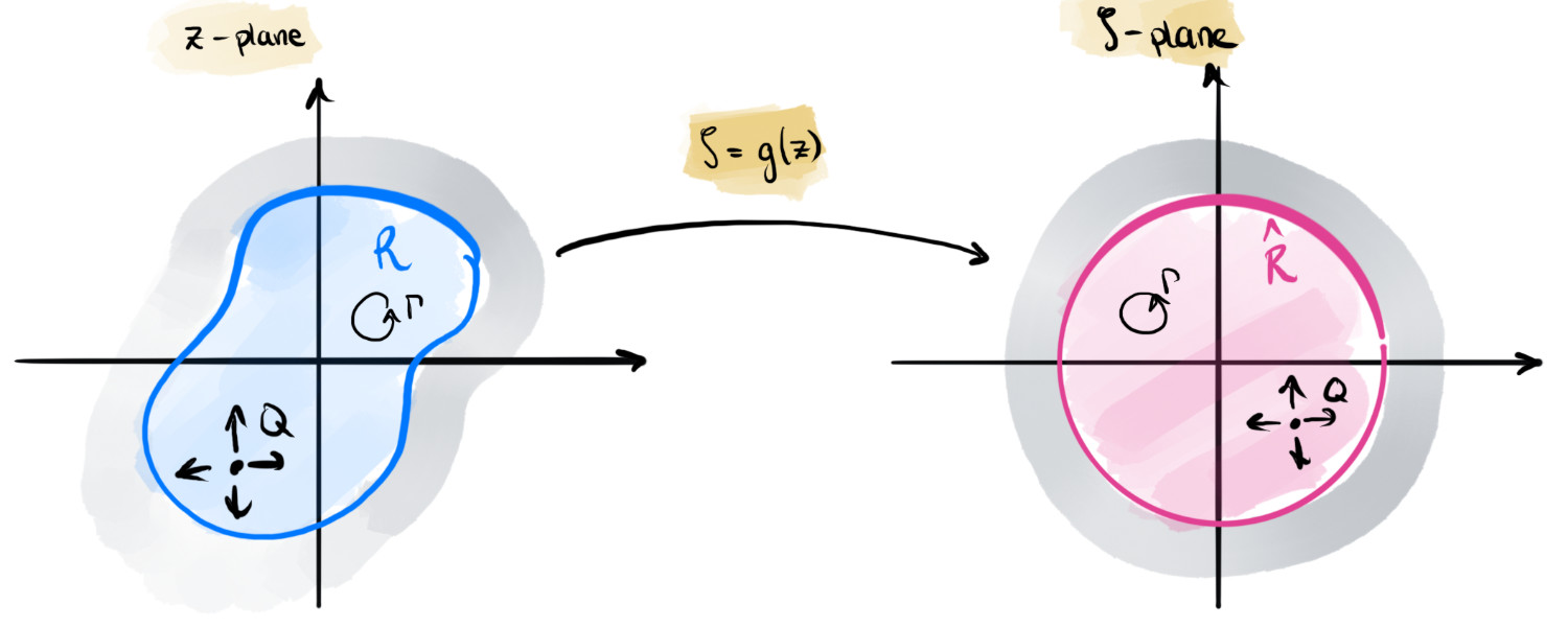
so that the region \(R\) is mapped to a new region \(\hat{R} \subseteq \mathbb{C}\text{,}\) as shown in Figure 4.5.1.
The hope is that within the \(\zeta\)-plane, the fluid region is sufficiently simple that a complex potential, say \(F(\zeta)\text{,}\) can be found. This task is aided by virtue of the fact that sinks/sources and vortices are preserved by the conformal map. Typically, we wish for \(\hat{R}\) to be e.g. the upper half-plane or the unit disc, with \(\partial\hat{R}\) to be the real axis or circumferance of the unit disc, respectively. Once found, the complex potential in the \(z\)-plane is then obtained simply by inverting the conformal map, i.e.
Figure4.5.1.A general conformal mapping from the \(z\)-plane to the \(\zeta\)-plane. The object is to map the region \(R\) to the region \(\hat{R}\text{,}\) which is geometrically simpler.
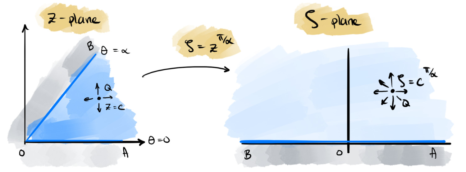
Consider fluid contained in a wedge with walls at \(\theta = 0\) and \(\theta = \alpha > 0\text{,}\) and with the fluid in \(0 < \theta < \alpha\text{.}\) A source of strength \(Q\) is placed somewhere within the flow, say at the point \(z = c\text{.}\)
It can be verified that this map transforms the fluid region to the upper half-\(\zeta\)-plane. Indeed the ray \(\theta = 0\) is mapped to the positive real axis and the ray \(\theta = \alpha\) is mapped to the negative real axis. This is shown in Figure 4.5.2.
In the \(\zeta\)-plane, the fluid problem thus consists of solving for flow in the upper half-plane with a source of strength \(Q\) at the location \(\zeta = c^{\pi/\alpha} = \zeta_c\text{,}\) with an impermeable boundary on the real \(\zeta\)-axis. Indeed, from the previous section, we know this can be solved using the method of images, with a source placed at both the point \(\zeta_c\) and its complex conjugate point, \(\overline{\zeta_c}\text{.}\) It then follows that the complex potential is
Let us specifically define a conformal map as a mapping, \(\zeta = g(z)\text{,}\) where \(g\) is analytic in a region \(R\) and also that \(\dd{g}{z} \neq 0\) in \(R\text{.}\)
If the boundary \(\partial{\hat{R}}\) is a streamline in the \(\zeta\)-plane, then the corresponding boundary \(\partial R\) is a streamline in the \(z\)-plane (and vice versa).
A source (or vortex) of strength \(Q\) at \(\zeta = g(c) \in \hat{R}\) in the \(\zeta\)-plane corresponds to a source (or vortex) of the same strength \(Q\) at \(z = c \in R\) in the \(z\)-plane (and vice versa).
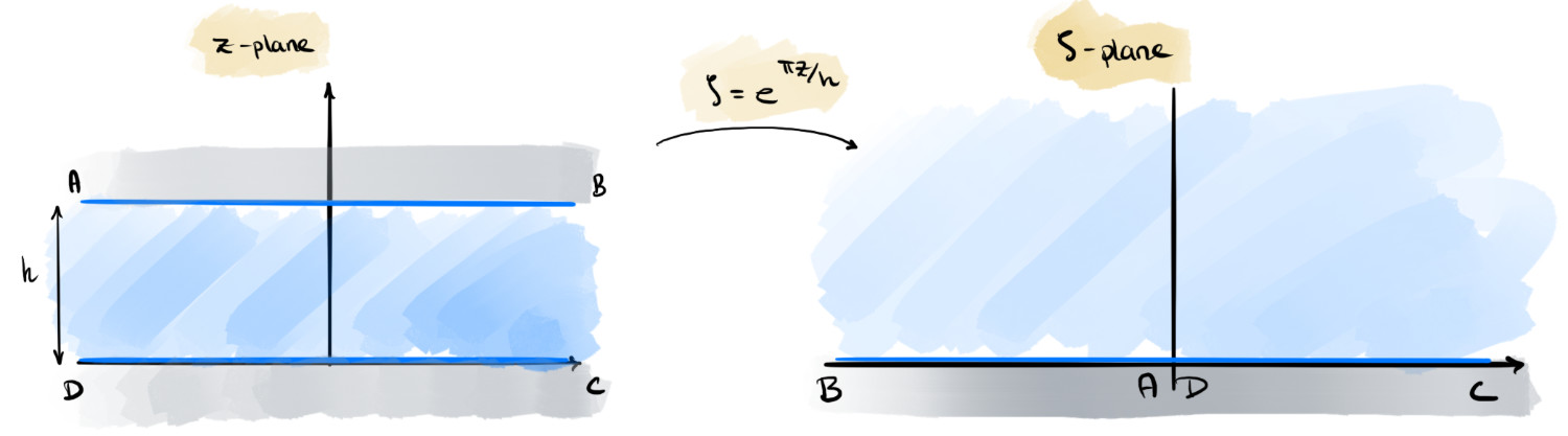
The exponential map is used to map a channel to a half-space. Consider a channel of width \(h\) in the region \(0 < \Im z < h\) in the \(z\)-plane. Then
maps this channel to the upper half-\(\zeta\)-plane. The correspondence of critical points and points at infinity in the pre-image and the image is shown in (4.5.4). It is good to see the map as essentially ’unfolding’ the infinite channel, sending points AD to the origin, while sending B to negative infinity and C to positive infinity. The conformal map will preserve the orientation of the boundary, so as we traverse along ABCD, the fluid region is always on the left.
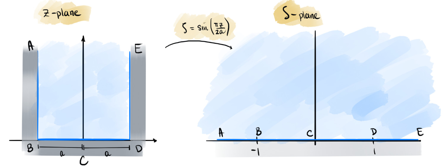
Trigonometric maps are used to map semi-infinite channels into a half space. Consider for example, the region \(R\) given in the following diagram in (4.5.5). We can then see that the semi-infinite channel of width \(2a\) has been mapped to the upper half-plane. The two corners at \(z = \pm a\) have been mapped to \(\zeta = \pm 1\text{,}\) respectively.
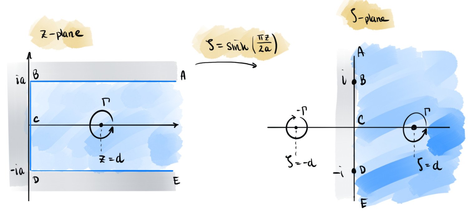
Example4.5.7.Vortex flow in a semi-infinite channel.
Consider the channel shown in the left of Figure 4.5.8. Insert a vortex of strength \(\Gamma\) at the point \(z = d \in \mathbb{R^+}\text{.}\) Verify that an appropriate conformal map is given by