As evidenced by the quotation above, during the great Victorian era, Lord Kelvin had predicted that the field of hydronamics (predominantly, the study of liquids) would reign over all the physical sciences. Today that is not quite true, in the sense that hydrodynamics is only one of many sub-branches of the wider study of fluid motion. However, Kelvin’s prediction is certainly true in spirit: there are very few branches in the physical sciences, from biology and chemistry, to engineering and physics, where the study of fluid mechanics does not possess strong historical and scientific connections. The principles, language, and techniques of fluid mechanics begin from the fundamental laws of conservation; in their form, one can argue that all of nature can be derived---this grandiose point is, to some extent, what Kelvin had meant when he referred to being the "root of all physical science".
Moreover, countless areas of mathematics, from the 19th century and onwards, have been developed as a direct consequence of the need to investigate the beautiful nature of fluid motion. These include everything from the theory of ordinary and partial differential equations, calculus, complex analysis, mathematical methods and approximation theory, geometry and topology, analysis, numerical methods and numerical analysis, industrial and applied mathematics, and so forth and so on.
In general, fluid mechanics includes both "statics" (fluids at rest) and "dynamics" (things in motion). This is a distinction that, in the authors’ opinions, mathematicians rarely use (we probably refer to "fluid mechanics" more commonly so as to avoid being specific); these distinctions are perhaps more important in engineering. For example, the study of the shape of a soap film or bubble between a wire hoop is a question of statics; but the behaviour of the soap or bubble if it moves or pops is a question of dynamics!
Fluid Mechanics
 ├── Fluid Statics
 │     ├── Hydrostatics → Pressure in tanks and dams
 │     ├── Buoyancy → Ship and submarine design
 │     └── Manometry → Pressure measurement in pipelines
 │
 └── Fluid Dynamics
       ├── Inviscid Flow
       │     ├── Potential Flow → Aerodynamics of airfoils
       │     └── Compressible Flow (ideal gases) → Supersonic jet nozzles
       │
       ├── Viscous Flow
       │     ├── Internal Flows (pipe/duct flow) → Water distribution networks
       │     ├── External Flows (boundary layers) → Drag on cars and airplanes
       │     └── Lubrication Theory → Bearings in machines
       │
       ├── Turbulence
       │     ├── Atmospheric Turbulence → Weather prediction
       │     └── Industrial Turbulence → Mixing in chemical reactors
       │
       └── Multiphase Flow
             ├── Gas–Liquid Flow → Oil & gas pipelines
             ├── Liquid–Solid Flow → Slurry transport in mining
             └── Gas–Solid Flow → Fluidized bed reactors
It is not uncommon for some scientists and mathematicians to devote their entire careers to an entire subbranch of fluid mechanics. Some university departments will focus solely on certain subbranches as well! Hence fluid mechanics is for many, a lifelong pursuit!
Euler’s equation relates the velocity of a fluid, \(\bu\text{,}\) with its density \(\rho\text{,}\) pressure \(p\text{,}\) and associated forces, \(\bg\text{.}\) It is an expression of the conservation of momentum of fluid, and is completed with an accompanying equation for conservation of mass. Together, the two equations are solved with the specification of additional boundary conditions to describe many liquids, from the water in your bathtub, to the water in the ocean as a ship travels through the surface.
Slowly, we will begin to appreciate the use of conservation laws, and the mathematics necessary, to derive the above equations (compressing some hundred years of scientific work into only a handful of lectures!). We will also appreciate that, despite their compact form, the above equations are certainly not easy to solve!
Our next task, starting in Chapter 4 is to study a particular simplification of the Euler equation that yields the flow of an ideal or potential fluid. Under such constraints, instead of solving the above difficult equations, we solve a much simpler equation:
for a so-called velocity potential, \(\phi\text{,}\) related to the velocity by \(\bu = \nabla \phi\text{.}\) Potential flow theory would have occupied some of the greatest minds of our time, from Euler, Lagrange, Bernoulli, d’Alembert, and Laplace of the 18th century; to the great Victorian scientists of the 19th century: Kelvin, Green, Stokes, Helmholtz; then towards the modern 20th century workers such as Prandtl, Lighthill, Milne-Thompson, and so forth. It is the simplest framework for studying the motion of a liquid, such as water, but enjoys incredibly deep connections with the beautiful theory of complex variables. We will study some of these connections, leading to learning about things such as conformal mapping theory.
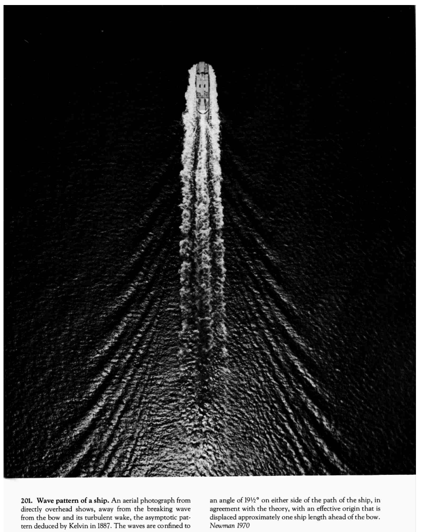
Figure1.0.3.In 1887, Kelvin famously predicted that the waves trailing a ship produce a wedge of approximately \(2 \times 19.5^\circ\text{.}\) This theory belongs to the analysis of linear water waves (though it is unlikely we will have time to reproduce Kelvin’s approximation!) From Van Dyke, An Album of Fluid Motion.
Water waves is probably the application that was at the forefront of Lord Kelvin’s thoughts when he discussed the state of hydrodynamics in the quotation that begins in Chapter 5. The study of the surface motion of water introduces a seemingly minor complexity that is responsible for great heartache: the fluid is now bounded by an unknown free surface, which much now be solved as part of the problem! The theory of water waves was at the heart of many minds in the 19th century, given its importance in all applications naval and oceanic. The study of water waves begins with so-called linear wave theory, and moves towards numerical solutions of the full Euler equations.
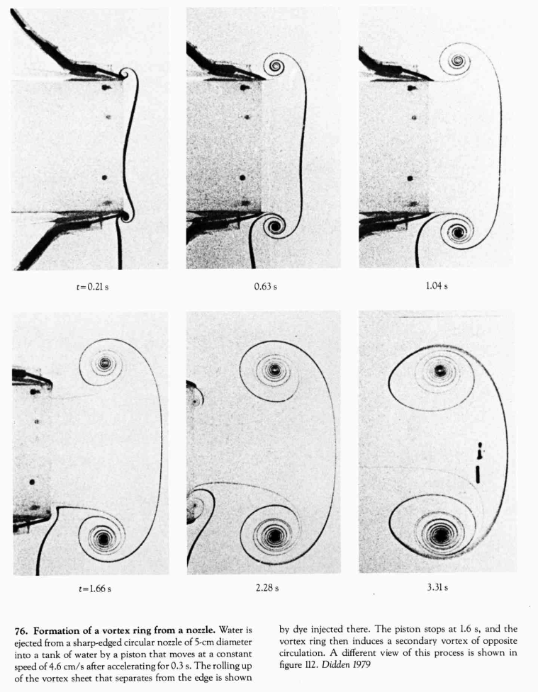
In the above applications, our attention will be focused on so-called irrotational flows: flows that either do not contain or do not introduce new rotational characteristics. Of course, real life fluids are rarely so well-behaved and indeed, the study of vortices is an important domain in its own right, leading to models for tornados, flight, and many other fluid phenomena. The principle character of Chapter 6 is the vorticity, \(\omega = \nabla \times \bu\text{.}\) What is vorticity, how does one measure it, and what is its role in governing fluid motion: these are the topics of this chapter.
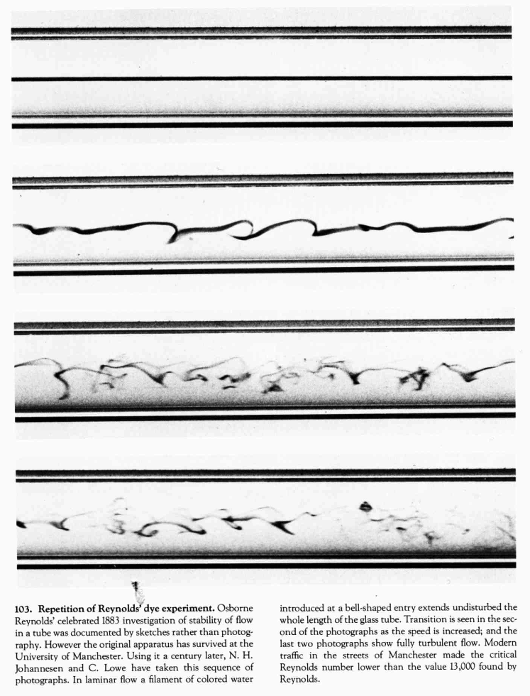
Figure1.0.5.As illustrated in Figure 0.0.1, in 1883 Rayleigh performed a famous experiment of stability of flow in a tube, showing the emergence of an instability as the speed of the flow is increased. This leads to turbulence, which is predicted, in principle, from the Navier-Stokes equations of viscous flows. (From Van Dyke, An Album of Fluid Motion.
Finally, the last part of this course will open up to the important discpline of viscous flows in Chapter 7. For this, the Euler equations are no longer sufficient, and we must include a dissipative component,
with \(\mu\) being the viscosity of the fluid. The above equation, together with an equation for conservation of mass, forms the so-called Navier-Stokes equations. All fluids are viscous to some extent, though some moreso than others. You will learn about the connections between viscous flow theory and inviscid theory, and some of the simple viscous flows that are foundational in this subbranch.