The main function of this chapter was to briefly review complex functions and also review/introduce you to the notion of branch cuts. Complex functions will be used in the potential theory of Chapter 4 and wave theory of Chapter 5.
Consider a contour that starts from \(z = 1\text{,}\) then encircles the origin (anticlockwise) and returns to \(z = 1\text{.}\) What is the jump in the value of \(f(z)\) at the end of the contour as compared to the start?
Let \(z = \e^{\im \theta}\text{.}\) For \(\theta = 0\text{,}\)\(f(z) = r^{1/2}\) if we choose the positive branch of the square root (by convention). At the other side of the branch cut, \(\theta = 2\pi\) and \(f(z) = r^{1/2} \e^{\pi \im} = -r^{1/2}\text{.}\) Therefore there is a jump in value of \(-2r^{1/2}\text{.}\)
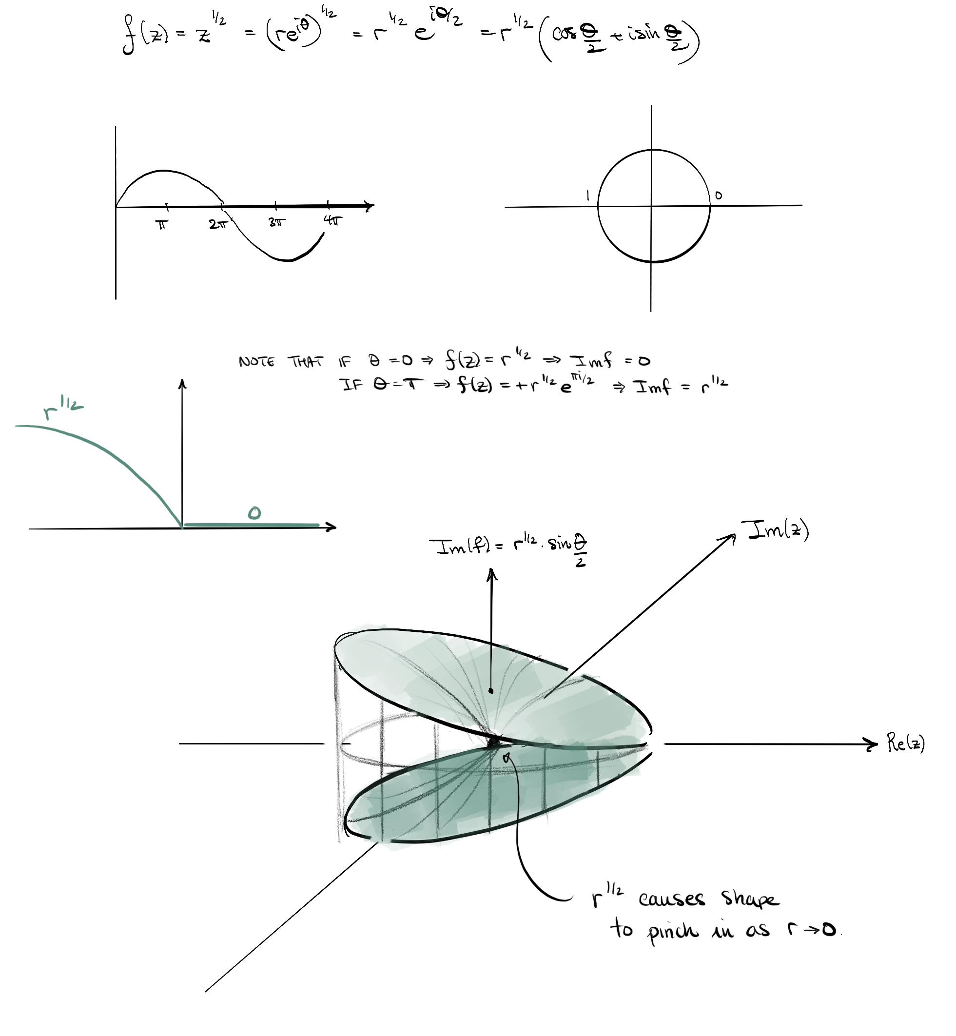
By hand, plot the Riemann surface as visualised in \((x, y, \Im f(x + \im y))\)-space, where \(\Im f(z) = r^{1/2} \sin(\theta/2)\text{.}\) You may also confirm your sketch with a computational tool, if desired.
It is useful to first consider the plot of \(\sin(\theta/2)\text{,}\) and then separately, what happens for the magnitude variation that depends on \(r^{1/2}\text{.}\)
A sketch of the imaginary part of the square root function is shown below. The two key features to capture is the dependence on \(\theta\) and the dependence on \(r\text{.}\)
Choose the branch cut from \(z = 1\) in the positive real direction. Choose the branch cut from \(z = -1\) in the negative real direction. Write either \(z = r_1
\e^{\im\theta_1}\) or \(z = r_2 \e^{\im\theta_2}\) for \(\theta_1\) and \(\theta_2\) defined as relative angles from the two branch points.
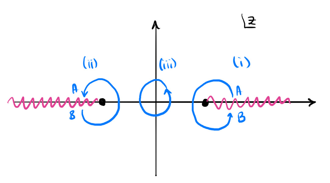
Show that: (i) when \(z = 1\) is encircled by a complete revolution, the function jumps in value by a factor of \(\e^{\im \pi}\text{;}\) (ii) that there is a similar jump in value when \(z = -1\) is encircled. Finally what happens if (iii) \(z = 0\) is encircled?
Let \(\theta_1 \in [0, 2\pi)\) be the angle about the point \(z = 1\text{.}\) Similarly let \(\theta_2 \in [-\pi, \pi)\) be the angle about the point \(z = -1\text{.}\)
Considering firstly a revolution around \(z = 1\) (that does not also enclose \(z =
-1\)). Let the initial point be denoted "A", with \(\theta_1 = 0, \theta_2 = 0\text{.}\) And the final point be "B", with \(\theta_1 = 2\pi\) and \(\theta_2 = 0\text{.}\)
(ii) We would similarly verify that for a contour around the branch point \(z = -1\) there is a jump. Let the initial point be denoted "A" with \(\theta_1 = \pi, \theta_2 =
-\pi\text{.}\) And the final point be "B" with \(\theta_1 = \pi, \theta_2 = \pi\text{.}\) Then
(iii) For the centre point, there are two cases to consider. The first case is if only \(z
= 0\) is encircled and none of the other branch points. This was the situation originally envisioned in the question. For example, consider the circle of radius 1/2, i.e. \(z = (1/2) \e^{\im \theta}\) with \(\theta \in [0, 2\pi)\text{.}\) You can verify that for this circle the start and end points agree.
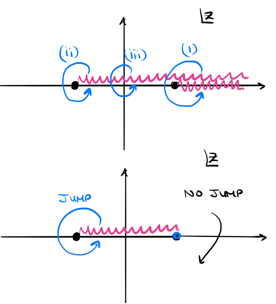
If along with \(z = 0\text{,}\) one of the branch points is encircled, then there would be a discontinuity. If both branch points are encircled, there is no discontinuity.
Figure1.3.2.Branch cut configuration for the double square root. The original choice of branches is shown on top. Through the analysis, we see that a circle (i) around \(z =
1\) does not produce a discontinuity. Hence only the second picture of the cut arrangement is needed.
Consider now a branch cut from \(z = -1\) that tends in the positive real direction and the branch cut from \(z = 1\) tends in the positive real direction as well. Repeat the experiment above, considering (i)-(iii). Conclude that there is no jump in value along the region \(z > 1\) and hence the branch cuts required only extends between \(z = \pm 1\text{.}\)
For this situation, we would define the ranges of \(\theta_1 \in [0, 2\pi)\) and \(\theta_2
\in [0, 2\pi)\text{.}\) One main difference is the analysis around the point \(z = 1\text{.}\) Consider the similar loop to the above with,
In essence, because both branch cuts are running in the positive real direction, when we orbit across \(z > 1\text{,}\) we jump through both branches, hence returning to the original. There is no required branch cut for \(z > 1\text{.}\)
The analysis of parts (ii) and (iii) are identical, with the exception of the angle range. However, the final result, of whether there exists a jump is the same.
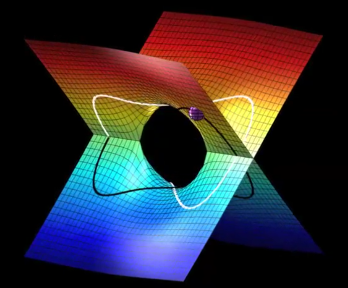
(Challenging). If you consider a plot of \((x, y, \Re f(x + \im y))\) or \((x, y,
\Im f(x + \im y))\text{,}\) what will the Riemann surface look like? You can attempt to plot this using any tool.
This is certainly not an easy function to imagine! There are two features you may want to keep in mind. First, in examining the imaginary part of the function, if \(z > 1\) on the real axis, then the imaginary part is zero. Second, if \(z < -1\) on the real axis, then again the function is zero. Finally, for the case of the branch selection in part (b), the there is a cut along \([-1, 1]\text{.}\) A generated plot is shown below for the imaginary part.
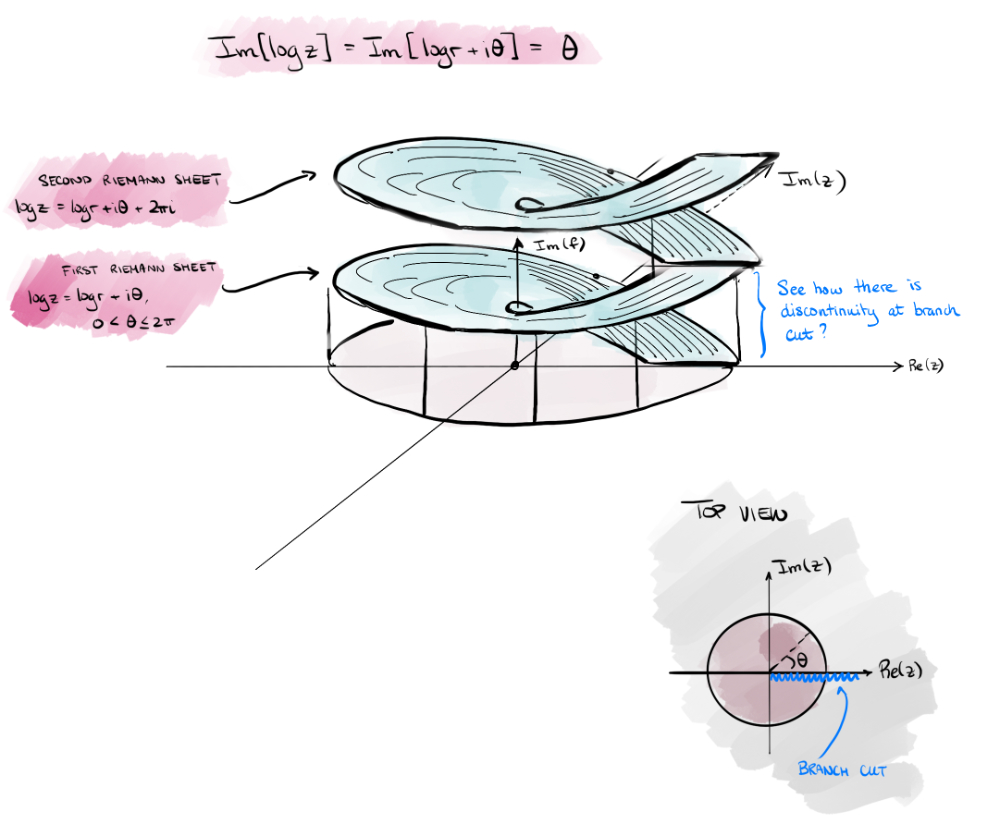
Take the branch cut along the positive real axis. Do your best to draw the Riemann surface (consisting of the distinct Riemann sheets) of the logarithm, as visualised in the space \((x, y, \Im f(x + \im y))\text{.}\)