Newtonian fluids

Section 7.4 Newtonian fluids

In this section we define an important class of fluids called Newtonian fluids. Many common fluids, including water and air, may be described as Newtonian.

🔗

Subsection 7.4.1 Incompressible Newtonian fluids

Many common fluids may be well described as incompressible Newtonian fluids.

🔗

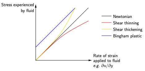
Definition 7.4.2. Incompressible Newtonian fluid.

We can define a Newtonian fluid by stating its constitutive relationship.

\begin{equation} \sigma_{ij}=-p\delta_{ij} +\mu\left(\pd{u_j}{x_i}+\pd{u_i}{x_j}\right),\tag{7.4.1} \end{equation}

where \(\mu\) is the dynamic shear viscosity. Alternatively, in vector form,

\begin{equation} \bsigma=-p\bI+2\mu\be,\tag{7.4.2} \end{equation}

where \(\be\) is the rate-of-strain tensor,

\begin{equation*} \be=\left(\begin{matrix} e_{11}&e_{12}&e_{13}\\ e_{21}&e_{22}&e_{23}\\ e_{31}&e_{32}&e_{33} \end{matrix}\right), \end{equation*}

where

\begin{equation} \be=\frac12\left(\nabla\bu+\left(\nabla\bu\right)^T\right) \quad\textrm{or}\quad e_{ij}=\frac12\left(\pd{u_j}{x_i}+\pd{u_i}{x_j}\right),\tag{7.4.3} \end{equation}

or, alternatively,

\begin{equation} \be=\left(\begin{array}{ccc} \pd{u}{x}&\frac12\left(\pd{u}{y}+\pd{v}{x}\right)&\frac12\left(\pd{u}{z}+\pd{w}{x}\right)\\ \frac12\left(\pd{u}{y}+\pd{v}{x}\right)&\pd{v}{y}&\frac12\left(\pd{v}{z}+\pd{w}{y}\right)\\ \frac12\left(\pd{u}{z}+\pd{w}{x}\right)&\frac12\left(\pd{v}{z}+\pd{w}{y}\right)&\pd{w}{z} \end{array}\right).\tag{7.4.4} \end{equation}

All three of these forms ((7.4.3) and (7.4.4)) are equivalent. Using (7.4.2), we may write the stress tensor of an incompressible Newtonian fluid in component form in Cartesian coordinates as

\begin{equation} \bsigma=\left(\begin{matrix} -p+2\mu\pd{u}{x}&\mu\left(\pd{u}{y}+\pd{v}{x}\right)&\mu\left(\pd{u}{z}+\pd{w}{x}\right)\\ \mu\left(\pd{u}{y}+\pd{v}{x}\right)&-p+2\mu\pd{v}{y}&\mu\left(\pd{v}{z}+\pd{w}{y}\right)\\ \mu\left(\pd{u}{z}+\pd{w}{x}\right)&\mu\left(\pd{v}{z}+\pd{w}{y}\right)&-p+2\mu\pd{w}{z} \end{matrix}\right).\tag{7.4.5} \end{equation}

🔗

Remark 7.4.3. Derivation of Newtonian fluid stress tensor from first principles.

Non-examinable:

🔗

Newtonian fluids have the following properties:

The deviatoric part of the stress tensor, \(\bd\text{,}\) is a linear function of the nine velocity gradients,

\begin{equation*} (\nabla\bu)_{ij}=\pd{u_j}{x_i}. \end{equation*}

This implies

\begin{equation*} d_{ij}=\sum_{l=1}^3\sum_{k=1}^3c_{ijkl}\pd{u_l}{x_k} \end{equation*}

for some unknown scalars \(c_{ijkl}\text{.}\)

🔗

🔗
The fluid is homogeneous, i.e. \(\bsigma\) does not depend explicitly on \(\bx\text{.}\) This implies that the \(c_{ijkl}\)’s are constant in space. An example of when this would not be the case would be an inhomogeneous fluid, such as a fluid that is heated differentially.
🔗

🔗
The fluid is isotropic, i.e. there is no preferred direction. Insisting that \(\bd\) transforms correctly under rotations (and in fact we only need to consider rotations through \(90^\circ\) about the coordinate axes) implies that \(c_{ijkl}\) is zero unless each subscript appears an even number of times. That is, the only non-zero terms are \(c_{1111}\text{,}\) \(c_{2222}\text{,}\) \(c_{3333}\) (which must all be equal), and those \(c_{ijkl}\)’s in which two of the indices \(i\text{,}\) \(j\text{,}\) \(k\text{,}\) \(l\) are ’1’ and two indices are ’2’, also terms with two `2’s and two `3’s, and terms with two `1’s and two `3’s (and these obey certain equalities too). An example of when this would not be the case would be an anisotropic fluid, such as nematic liquid crystals (long chain molecules that align in a magnetic field) or flowing blood in which the red blood cells align in the direction of flow).
🔗

🔗

Additionally requiring that \(\bd\) is a symmetric matrix means that, in component form, we can reduce the \(c_{ijkl}\)’s down to just two independent scalar parameters, \(\lambda\) and \(\mu\text{,}\) and we have

\begin{equation} \sigma_{ij}=-p\delta_{ij}+\lambda\delta_{ij}\sum_{k=1}^3\pd{u_k}{x_k} +\mu\left(\pd{u_j}{x_i}+\pd{u_i}{x_j}\right),\tag{7.4.6} \end{equation}

where \(\lambda\) is the bulk viscosity of the fluid and \(\mu\) is the dynamic shear viscosity. In vector form

\begin{equation*} \bsigma=-p\bI+\lambda\left(\nabla\cdot\bu\right)\bI+2\mu\be, \end{equation*}

where \(\be\) is the rate-of-strain tensor, given by

\begin{equation*} \be=\left(\begin{matrix} e_{11}&e_{12}&e_{13}\\ e_{21}&e_{22}&e_{23}\\ e_{31}&e_{32}&e_{33} \end{matrix}\right). \end{equation*}

If the fluid is incompressible, then \(\nabla\cdot\bu=0\) and the bulk viscosity is undefined, meaning that (7.4.6) reduces to (7.4.1).

🔗

Remark 7.4.4. Formula in cylindrical and spherical coordinates.

In cylindrical polar coordinates the rate-of-strain tensor is given by

\begin{equation} \be=\left(\begin{matrix} \pd{u_r}{r}&\frac12\left(r\pd{(u_\theta/r)}{r}+\frac1r\pd{u_r}{\theta}\right)&\frac12\left(\pd{u_z}{r}+\pd{u_r}{z}\right)\\ \frac12\left(r\pd{(u_\theta/r)}{r}+\frac1r\pd{u_r}{\theta}\right)&\frac1r\pd{u_\theta}{\theta}+\frac{u_r}{r}&\frac12\left(\pd{u_\theta}{z}+\frac1r\pd{u_z}{\theta}\right)\\ \frac12\left(\pd{u_z}{r}+\pd{u_r}{z}\right)&\frac12\left(\pd{u_\theta}{z}+\frac1r\pd{u_z}{\theta}\right)&\pd{u_z}{z} \end{matrix}\right),\tag{7.4.7} \end{equation}

and in spherical polar coordinates it is

\begin{equation} \be=\left(\begin{matrix} \pd{u_r}{r}&\frac12\left(r\pd{(u_\theta/r)}{r}+\frac1r\pd{u_r}{\theta}\right)&\frac12\left(r\pd{(u_\phi/r)}{r}+\frac1{r\sin\theta}\pd{u_r}{\phi}\right)\\ \frac12\left(r\pd{(u_\theta/r)}{r}+\frac1r\pd{u_r}{\theta}\right)&\frac1r\pd{u_\theta}{\theta}+\frac{u_r}{r}&\frac12\left(\frac1{r\sin\theta}\pd{u_\theta}{\phi}+\frac{\sin\theta}{r}\pd{(u_\phi/\sin\theta)}{\theta}\right)\\ \frac12\left(r\pd{(u_\phi/r)}{r}+\frac1{r\sin\theta}\pd{u_r}{\phi}\right)&\frac12\left(\frac1{r\sin\theta}\pd{u_\theta}{\phi}+\frac{\sin\theta}r\pd{(u_\phi/\sin\theta)}{\theta}\right)&\frac1{r\sin\theta}\pd{u_\phi}{\phi}+\frac{u_r+u_\theta\cot\theta}{r} \end{matrix}\right).\tag{7.4.8} \end{equation}

You do not need to know these matrices for this course. You might have to use them, but these formulae would be supplied. You do need to know the Cartesian equivalent (7.4.4).

🔗

Remark 7.4.5. Notes on the Newtonian fluids stress tensor.

For an incompressible Newtonian fluid the stress tensor has only one parameter, the shear viscosity, \(\mu\text{,}\) and there are are only two parameters needed to describe the mechanical behaviour of the fluid: \(\mu\) and the fluid density, \(\rho\text{.}\)
🔗

🔗
The shear viscosity, \(\mu\text{,}\) is often a function of temperature, and sometimes of pressure too. For most common fluids the shear viscosity decreases with increasing temperature.
🔗

🔗

🔗

Subsection 7.4.2 Stress at a surface

In Definition 7.3.3, we stated formulae for the stress that a fluid exerts on a rigid solid boundary. We are now in a position to check the formulae given there.

🔗

The normal stress on a surface with normal \(\bn\) is given by

\begin{equation} \left(\bsigma\bn\right)\cdot\bn =-p+2\mu\bn\cdot\nabla\left(\bu\cdot\bn\right).\tag{7.4.9} \end{equation}

The last term represents \(2\mu\) times the derivative of the normal component of the velocity in the normal direction. Thus the normal stress is not necessary equal to the pressure!

🔗

However, if we assume that the surface is fixed then we may show that the normal stress of an incompressible Newtonian fluid does equal the pressure:

By rotating the coordinate axes we may assume that \(\bn=\bi\text{.}\)
🔗

🔗
From (7.4.9), the normal stress is \(-p+2\mu\partial u/\partial x\text{.}\)
🔗

🔗
Since the fluid is incompressible,

\begin{equation*} \nabla\cdot\bu=\pd{u}{x}+\pd{v}{y}+\pd{w}{z}=0. \end{equation*}

🔗

🔗
The boundary conditions at the solid surface are \(u=v=w=0\text{.}\) Thus

\begin{equation*} \pd{v}{y}=\pd{w}{z}=0 \end{equation*}

on the surface. The continuity equation implies that

\begin{equation*} \pd{u}{x}=0 \end{equation*}

also.

🔗

🔗
Hence the normal stress on the surface is \(-p\text{.}\)
🔗

🔗

🔗

At a fixed solid surface the shear stress of a Newtonian fluid equals the viscosity multiplied by the derivative of the component of velocity parallel to the surface with respect to the perpendicular coordinate. We can show this as follows:

As before we may rotate the coordinate axes so that \(\bn=\bi\text{.}\)
🔗

🔗
Using (7.4.5), the stress at the surface is

\begin{equation*} \btau=\bsigma\bn =\left(\begin{matrix} -p+2\mu\pd{u}{x}\\ \mu\left(\pd{u}{y}+\pd{v}{x}\right)\\ \mu\left(\pd{u}{z}+\pd{w}{x}\right) \end{matrix}\right), \end{equation*}

and the shear stresses are given by the \(y\)- and \(z\)-components:

\begin{equation*} \tau_y=\mu\left(\pd{u}{y}+\pd{v}{x}\right),\quad \tau_z=\mu\left(\pd{u}{z}+\pd{w}{x}\right). \end{equation*}

🔗

🔗
No slip boundary conditions at the solid surface are \(u=v=w=0\text{.}\) Thus

\begin{equation*} \pd{u}{y}=\pd{u}{z}=0 \end{equation*}

on the surface.

🔗

🔗
Hence the shear stresses on the surface are

\begin{equation*} \tau_y=\mu\pd{v}{x}\quad\textrm{and}\quad\tau_z=\mu\pd{w}{x}, \end{equation*}

agreeing with the previous definitions.

🔗

🔗

🔗

Subsection 7.4.3 Inviscid fluids

In previous chapters in this course, you studied inviscid or ideal fluids. These are fluids with \(\mu=0\text{.}\) In this case, the constitutive law (7.4.5) becomes

\begin{equation} \bsigma=-p \bI=\left(\begin{matrix} -p&0&0\\ 0&-p&0\\ 0&0&-p \end{matrix}\right),\tag{7.4.10} \end{equation}

and thus the stress in the fluid is not affected by the fluid motion.

🔗

Subsection 7.4.4 Non-Newtonian fluids

Many fluids do not obey the assumptions underlying a Newtonian fluid, meaning that their constitutive relationship takes a more complicated form. Many foods and household products, e.g. egg white, custard, shampoo, toothpaste have a non-Newtonian rheology. In the case of foods, this is often because the non-Newtonian properties themselves lend a texture that makes them taste better! For household products the non-Newtonian properties help us use them (for example a Newtonian shampoo might drain off our hair before we have a chance to work it in).

🔗

The Navier–Stokes equations do not work for genuinely non-Newtonian flows, and the pressure and viscous terms must be replaced by a formula that captures the rheology. However, for a surprising variety of complex fluids, the Navier–Stokes equations do in fact provide a remarkably good description of the behaviour.

🔗

In general, however, the rheology of non-Newtonian fluids is often very complex, and is an area of active research. Categories include the following:

Non-constant viscosity: This is perhaps the simplest way a fluid can be non-Newtonian. Examples include shear thinning fluids, e.g. blood, and shear-thickening fluids, e.g. fluids containing cornflour such as custard, or fluids whose viscosity depends on the temperature of the fluid.
🔗

Figure 7.4.6. Examples of Non-Newtonian fluids
🔗
A short video on shear thickening fluids is both fun and educational.
🔗

🔗
Viscoelastic fluids: These are fluids that have both elastic and viscous properties, that is the molecules seem to have a memory and spring back when they are suddenly displaced (but not so much when they are slowly displaced); thus they are sometimes described as having a `fading memory’. In this case the formula for the deviatoric part of the stress tensor involves an integral over the previous states of the fluid. Examples include ketchup, paint, mucus and vitreous humour.
🔗

🔗
Anisotropic fluids: Some fluids respond differently to the same stress but applied in different directions. An example of this is blood, which contains red blood cells affecting the dynamics. When the blood is flowing the cells align, meaning the effective viscosity is much less in the direction of flow and more in the transverse direction (this is also related to the fact that blood is shear thinning). In large arteries it is usually acceptable to model blood as a Newtonian fluid because the diameter of the artery is many times that of the cells. However, for small arteries, such as that in Figure 7.4.7, the Newtonian model does not give an accurate picture.
🔗

Figure 7.4.7. Computer simulation of blood flow in a microvessel by the Biological Flow Studies Laboratory in Tohoku University, Japan. The left picture shows the view of the blood from the outside (with the vessel walls removed), whilst that on the right shows the view in the central plane of the vessel.
🔗
Figure 7.4.8 shows a schematic representation of nematic liquid crystals, which are used in computer displays, electronic signs etc. These align by themselves to a preferred direction for high enough temperatures, and a magnetic field can be used to set the direction.
🔗

Figure 7.4.8. Schematic representation of nematic liquid crystals, an example of an anisotropic fluid.
🔗
🔗

🔗

Subsection 7.4.5 examples

Example 7.4.9. Calculating the stress due to a shear flow.

Consider an incompressible Newtonian fluid flowing in \(y\geq0\) in Cartesian coordinates \((x,y,z)\) in a uniform pressure field \(p=p_0\) with \(p_0\) constant, and whose velocity components are respectively given by

\begin{equation*} u=ky,\quad v=0,\quad w=0, \end{equation*}

(it may be shown these satisfy the governing equations). Find the stress tensor at a general location. Hence find the stress at a general location on an imaginary surface with unit normal vector \(\bn=(n_x,n_y,0)\text{.}\) In this question you may neglect gravity.

🔗

Solution.

The stress tensor is given by

\begin{equation*} \bsigma=-p\bI+2\mu\be, \end{equation*}

where the rate-of-strain tensor \(\be\) is given by

\begin{equation*} \be=\left(\begin{matrix} \pd{u}{x}&\frac12\left(\pd{u}{y}+\pd{v}{x}\right)\\ \frac12\left(\pd{u}{y}+\pd{v}{x}\right)&\pd{v}{y} \end{matrix}\right) =\left(\begin{matrix}0&k/2\\k/2&0\end{matrix}\right). \end{equation*}

Hence the stress tensor \(\bsigma\) is given by

\begin{equation*} \bsigma=-p\bI+2\mu\be =\left(\begin{matrix}-p_0&k\mu\\k\mu&-p_0\end{matrix}\right). \end{equation*}

Thus for a general unit vector

\begin{equation*} \btau=\bsigma\bn =\left(\begin{matrix}-p_0&k\mu\\k\mu&-p_0\end{matrix}\right)\left(\begin{matrix}n_x\\n_y\end{matrix}\right) =\left(\begin{matrix}-p_0n_x+k\mu n_y\\k\mu n_x-p_0n_y\end{matrix}\right). \end{equation*}

Note:

For example with \(\bn=\bj\text{,}\) we have \(\btau=(k\mu,-p_0)\text{.}\) This makes sense as there is a background pressure \(p_0\) pressing into the surface and a stress \(k\mu\) arising from the shear flow and running along the surface. It also agrees with the formulae for stress at a surface given in Definition 7.3.3.
🔗

🔗
Likewise if \(\bn=\bi\text{,}\) we have \(\btau=(-p_0,k\mu)\text{.}\) This formula cannot be compared with the formula given in Definition 7.3.3 as it would not be possible to put in a rigid surface with normal \(\bn=\bi\) without changing the flow.
🔗

🔗

🔗

Example 7.4.11. Calculating the stress due to flow in a pipe.

We consider a flow of an incompressible Newtonian fluid in a circular cylinder of radius \(a\) and infinite length in the \(z\)-direction, working in cylindrical polar coordinates \((r,\theta,z)\) with axis along the cylinder axis. The velocity components are given by

\begin{equation*} (u_r,u_\theta,u_z)=\left(0,0,\frac{G}{4\mu}\left(a^2-r^2\right)\right), \end{equation*}

where \(G=-\partial p/\partial z\) is the axial pressure gradient. Find the stress tensor at a general point and comment on it. Note that this flow is a famous solution of the governing equations and is called Hagen–Poiseuille flow.

🔗

Solution.

We have the rate-of-strain tensor given by (7.4.7) as

\begin{align*} \be=&\left(\begin{matrix} \pd{u_r}{r}&\frac12\left(r\pd{(u_\theta/r)}{r}+\frac1r\pd{u_r}{\theta}\right)&\frac12\left(\pd{u_z}{r}+\pd{u_r}{z}\right)\\ \frac12\left(r\pd{(u_\theta/r)}{r}+\frac1r\pd{u_r}{\theta}\right)&\frac1r\pd{u_\theta}{\theta}+\frac{u_r}{r}&\frac12\left(\pd{u_\theta}{z}+\frac1r\pd{u_z}{\theta}\right)\\ \frac12\left(\pd{u_z}{r}+\pd{u_r}{z}\right)&\frac12\left(\pd{u_\theta}{z}+\frac1r\pd{u_z}{\theta}\right)&\pd{u_z}{z} \end{matrix}\right)\\ =&\left(\begin{matrix}0&0&-\frac{Gr}{4\mu}\\0&0&0\\-\frac{Gr}{4\mu}&0&0\end{matrix}\right) \end{align*}

and hence

\begin{equation*} \bsigma=-p\bI+2\mu\be =\left(\begin{matrix}-p&0&-\frac12Gr\\0&-p&0\\-\frac12Gr&0&-p\end{matrix}\right). \end{equation*}

Incompressibility requires \(G\) to be constant, and hence \(p=p_0-Gz\text{,}\) where \(p_0\) is a constant, and giving

\begin{equation*} \bsigma=\left(\begin{matrix}-p_0+Gz&0&-\frac12Gr\\0&-p_0+Gz&0\\-\frac12Gr&0&-p_0+Gz\end{matrix}\right). \end{equation*}

Hence for imaginary surfaces with normal vectors \(\hat{\boldsymbol{r}}\text{,}\) \(\hat{\boldsymbol{\theta}}\text{,}\) \(\hat{\boldsymbol{z}}\text{,}\) respectively, the stress on the surface is given by

\begin{align*} \btau_r=&\bsigma\hat{\boldsymbol{r}}=\left(Gz-p_0\right)\hat{\boldsymbol{r}}-\frac12Gr\hat{\boldsymbol{z}},\\ \btau_\theta=&\bsigma\hat{\boldsymbol{\theta}}=\left(Gz-p_0\right)\hat{\boldsymbol{\theta}},\\ \btau_z=&\bsigma\hat{\boldsymbol{z}}=\left(Gz-p_0\right)\hat{\boldsymbol{z}}-\frac12Gr\hat{\boldsymbol{r}}. \end{align*}

It is not possible to compare these formulae with the ones given in Definition 7.3.3. The exception is the case when we find the stress on the wall (\(r=a\)), which we can do by setting the normal vector \(\bn=-\hat{\boldsymbol{r}}\text{,}\) giving

\begin{equation*} \btau=-\bsigma\hat{\boldsymbol{r}}=\left(p_0-Gz\right)\hat{\boldsymbol{r}}+\frac12Ga\hat{\boldsymbol{z}}, \end{equation*}

that is a normal stress equal to minus the pressure and an axial shear stress \(Ga/2\) (which is \(-\mu\,\partial u_z/\partial r\text{,}\) as expected).

🔗

Prev Top Next