The method of images

Section 4.4 The method of images

The preceeding sections would give the misleading impression that solving potential-flow problems for two-dimensional flows is easy. This is not the case, and the primary reason is due to the presence of boundary conditions. The elementary flows we have previously considered were unconfined and/or we did not consider additonal constraints on their behaviours at infinity. In reality, a real physical fluid, whether in the ocean, the air, or in a container, is confined in some direction, and we must often consider subtle questions about the mechanism that produces the fluid motion.

🔗

In this section, we consider the situation of solving for the potential flow in a fluid region with boundaries. Recall that this is equivalent to finding a velocity potential satisfying $\nabla^2 \phi = 0$ or an analytic complex potential, $f(z)\text{.}$

🔗

Recall from Note 3.4.7 that on solid boundaries, we must impose the no-flux condition that

\begin{equation*} \bu \cdot \bn = \nabla \phi \cdot \bn = 0 \quad \text{on $\partial V$}. \end{equation*}

🔗

Subsection 4.4.1 Planar boundaries: a half-plane

Consider the situation illustrated in Figure 4.4.1.

🔗

Figure 4.4.1. A flow region in the right half-plane, with a single source placed at $x = d\text{.}$
🔗

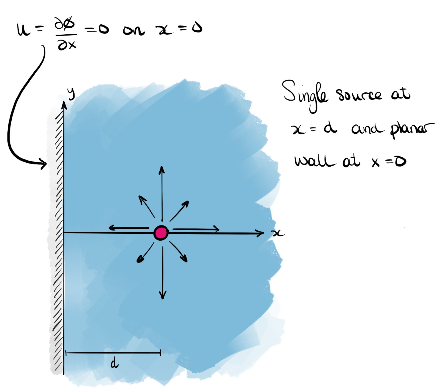
We envision a semi-infinite region of fluid bounded on the left by a wall at $x = 0\text{.}$ A single (line) source of strength $Q$ is placed at $x = d\text{.}$ Therefore from (4.3.5), we would expect that at least near $x = d\text{,}$ the complex potential behaves as

\begin{equation*} f(z) \sim \frac{Q}{2\pi} \log (z-d) \quad \text{as $z \to d$}. \end{equation*}

However the above solution does not satisfy the required boundary conditions at $x = 0$ since it corresponds to a velocity field for which the horizontal velocity penetrates through $x = 0\text{.}$ This can be verified via inspection. For example, we can inspect the velocity or the streamlines; this is part of Exercise 4.7.4.

🔗

Rephrased in terms of the streamlines, the boundary condition at $x = 0$ is equivalent to the constraint that

\begin{equation*} \Im f(z) = \psi = \textrm{constant at $x = 0$}. \end{equation*}

🔗

Our inspired solution to the above problem is referred to as the method of images.

🔗

Note 4.4.2. Method of images.

Given potential flow problem, we consider the superposition of elementary sinks/sources, i.e.

\begin{equation*} f(z) = \frac{1}{2\pi} \sum_{j=0}^{N-1} Q_j \log(z - z_j), \end{equation*}

and/or vortices,

\begin{equation*} f(z) = -\frac{\im}{2\pi} \sum_{j=0}^{N-1} \Gamma_j \log(z - z_j). \end{equation*}

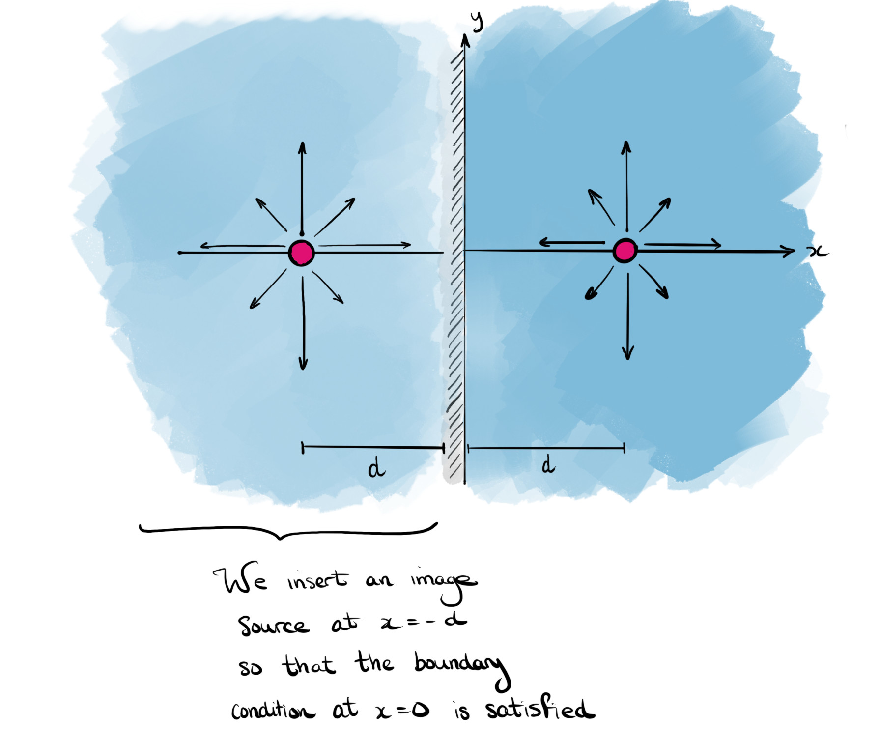
The strengths and locations of the individual contributions are chosen so that boundary conditions on the required boundaries (including at infinity) can be met.

🔗

Notice that the linearity of the potential flow problem is crucial: any analytic function is associated with a velocity potential that satisfies Laplace’s equation, $\nabla^2 \phi = 0\text{,}$ and therefore the superposition of such functions also yields a permissible complex potential, $f\text{.}$

🔗

We consider the addition of a "fictitious" image source, with the same strength at the reflected point $x = -d\text{,}$ which lies outside of the posited fluid region. This gives the complex potential of

\begin{equation*} f(z) = \frac{Q}{2\pi} \log(z - d) + \frac{Q}{2\pi} \log(z + d). \end{equation*}

This yields the illustration of the flow in Figure 4.4.3

🔗

Figure 4.4.3. Placement of the image source at $x = -d$ makes it so the boundary condition on $x = 0$ can be satisfied.
🔗

The corresponding complex velocity is given by

\begin{equation*} u - \im v = f'(z) = \frac{Q}{2\pi}\frac{z}{z^2 - d^2}. \end{equation*}

So indeed, on the central boundary, we have $z = \im y\text{,}$ and

\begin{equation*} u - \im v = - \im \frac{Q}{\pi} \frac{y}{y^2 + d^2}, \end{equation*}

and the velocity is entirely vertical. So indeed, the condition that $\bu \cdot \bn = 0$ on the planar boundary is satisfied.

🔗

In order to study the complex velocity, $f(z)\text{,}$ and develop an equation for the streamlines of the flow, we must first navigate the fact that the complex logarithm function is only well-defined in a slit complex plane. First, let

\begin{equation*} z - d = r_1 \e^{\im \theta_1} \quad \textrm{and} \quad z + d = r_2 \e^{\im \theta_2}. \end{equation*}

Using the definition of the complex logarithm (4.3.6), we have

\begin{equation*} f(z) = \frac{Q}{2\pi} \left[ \log r_1 + \log r_2\right] + \im \frac{Q}{2\pi}\left[ \theta_1 + \theta_2 \right]. \end{equation*}

The definitions of $r_1, r_2$ and $\theta_1, \theta_2\text{,}$ are shown in the below figure. In order for each logarithm to be well defined, the angles $\theta_1$ and $\theta_2$ must be restricted to be less than a complete revolution. We thus restrict $\theta_1 \in [0, 2\pi)$ and $\theta_1 \in [-\pi, \pi)\text{.}$

🔗

Figure 4.4.4. When considering the evaluation of the flow, we must take care of the fact that the logarithm is multi-valued. A branch cut from each of the two branch points is imposed.
🔗

In Exercise 4.7.5, you will be asked to develop an equation for the streamlines of this flow.

🔗

The above ideas can be extended to the situation of a line vortex in a half plane. Again, we are interested in describing the flow due to a line vortex at $z = d\text{,}$ and therefore we expect that near this point,

\begin{equation*} f(z) \sim -\frac{\im\Gamma}{2\pi} \log(z - d) \quad \textrm{as $z \to d$}. \end{equation*}

However, the above potential does not satisfy the necessary zero-flux condition at $x = 0\text{.}$

🔗

In this case, the approach is to add an image vortex at $z = -d\text{,}$ but opposite in direction:

\begin{equation*} f(z) = -\frac{\im\Gamma}{2\pi} \log(z - d) + \frac{\im\Gamma}{2\pi} \log(z + d). \end{equation*}

Therefore, this flow is composed by a line vortex circulating anticlockwise on the right, and a line vortex circulating clockwise on the left. It can be verified that the complex velocity is given by

\begin{equation*} u - \im v = -\frac{\im \Gamma d}{\pi(z^2 - d^2)} \end{equation*}

and indeed the velocity at $x = 0$ is entirely vertical and there is no flux through the boundary.

🔗

There is an exercise in Exercise 4.7.6.

🔗

Remark 4.4.5. Uniqueness of solutions.

You may be wondering: if a permissible potential function is found that satisfies the necessary boundary conditions, can we be certain it is the unique solution in the problem (up to a constant)? You may understand the construction of potentials, via the method of images, but perhaps irked that it involves the insertion of these so-called ’fictitious’ points. The answer, at least for most non-pathological problems in potential flow theory (i.e. all the problems you study) is yes, the solution you have found is assured to be the only solution (up to a constant).

🔗

This is, to some extent, related to the uniqueness of analytic continuation. In a nutshall, the relevant theorem states that given two admissible complex potentials, say $f_1(z)$ and $f_2(z)\text{,}$ that agree on the line $x = 0$ (in the case of the above situation), it is the case that $f_1 = f_2$ everywhere (where they are analytic).

🔗

Therefore, you can be certain that solutions you find via the trick of method of images are the only solutions.

🔗

Prev Top Next