Skip to main content \(\renewcommand*{\Re}{\operatorname{Re}}
\renewcommand*{\Im}{\operatorname{Im}}
\newcommand{\e}{\mathrm{e}}
\newcommand{\im}{\mathrm{i}}
\newcommand{\de}{\mathrm{d}}
\newcommand{\dd}[2]{\frac{\de#1}{\de#2}}
\newcommand{\DD}[2]{\frac{\mathrm{D}#1}{\mathrm{D}#2}}
\newcommand{\pd}[2]{\frac{\partial#1}{\partial#2}}
\newcommand{\pD}[2]{\dfrac{\partial#1}{\partial#2}}
\newcommand{\pdd}[2]{\frac{\partial^2\!#1}{\partial#2^2}}
\newcommand{\dxyz}{\de{x}\de{y}\de{z}}
\newcommand{\dXYZ}{\de{X}\de{Y}\de{Z}}
\newcommand{\bx}{\boldsymbol{x}}
\newcommand{\bs}{\boldsymbol{s}}
\newcommand{\be}{\boldsymbol{e}}
\newcommand{\bX}{\boldsymbol{X}}
\newcommand{\bn}{\boldsymbol{n}}
\newcommand{\bt}{\boldsymbol{t}}
\newcommand{\bu}{\boldsymbol{u}}
\newcommand{\bv}{\boldsymbol{v}}
\newcommand{\ba}{\boldsymbol{a}}
\renewcommand{\bf}{\boldsymbol{f}}
\newcommand{\bg}{\boldsymbol{g}}
\newcommand{\bF}{\boldsymbol{F}}
\newcommand{\bomega}{\boldsymbol{\omega}}
\newcommand{\bOmega}{\boldsymbol{\Omega}}
\newcommand{\bsigma}{\boldsymbol{\sigma}}
\newcommand{\btau}{\boldsymbol{\tau}}
\newcommand{\bd}{\boldsymbol{d}}
\newcommand{\bI}{\boldsymbol{I}}
\newcommand{\bi}{\boldsymbol{i}}
\newcommand{\bj}{\boldsymbol{j}}
\newcommand{\bk}{\boldsymbol{k}}
\newcommand{\br}{\boldsymbol{r}}
\renewcommand{\bt}{\boldsymbol{t}}
\newcommand{\btheta}{\boldsymbol{\theta}}
\newcommand{\bphi}{\boldsymbol{\phi}}
\newcommand{\bz}{\boldsymbol{z}}
\newcommand{\bq}{\boldsymbol{q}}
\newcommand{\bzero}{\boldsymbol{0}}
\newcommand{\bnabla}{\boldsymbol{\nabla}}
\DeclareGraphicsRule{.gif}{png}{.png}{}
\newcommand{\lt}{<}
\newcommand{\gt}{>}
\newcommand{\amp}{&}
\definecolor{fillinmathshade}{gray}{0.9}
\newcommand{\fillinmath}[1]{\mathchoice{\colorbox{fillinmathshade}{$\displaystyle \phantom{\,#1\,}$}}{\colorbox{fillinmathshade}{$\textstyle \phantom{\,#1\,}$}}{\colorbox{fillinmathshade}{$\scriptstyle \phantom{\,#1\,}$}}{\colorbox{fillinmathshade}{$\scriptscriptstyle\phantom{\,#1\,}$}}}
\)
Preface Official description
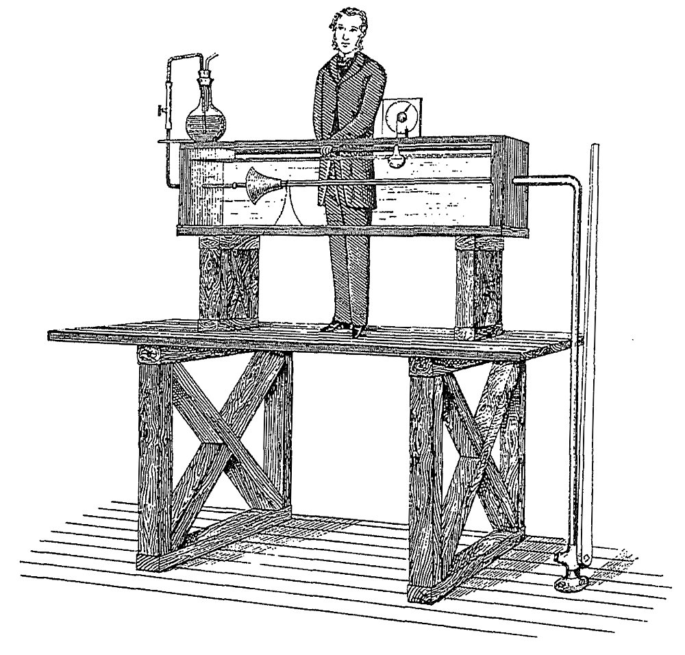
Figure 0.0.1. Rayleigh’s 1883 experiment on turbulence, as duplicated in World of Flosws (Darrigol, 2005).
Aims
In this unit you will explore the mathematical theory of fluid dynamics, with a view towards applications to physical phenomena such as flight, vortex motion and water waves. You will study the mathematics of conservation laws and the derivation of governing fluid dynamical equations. This unit will provide you with a foundation for further study of more advanced theory of fluid dynamics and continuum mechanics, and its application in scientific areas including engineering, physics and biology.
Outcomes
(i) Demonstrate an understanding of the principles of mathematical fluid dynamics; (ii) discuss and apply techniques from vector calculus and complex variable theory to analyse and solve fluid flow problems; (iii) give a qualitative and quantitative account of a range of phenomena in fluid dynamics.
Content
Complex analysis primer: Cauchy-Riemann equations; harmonic functions; complex maps; residue integration. The mathematics of fluid phenomena and its applications: derivation and interpretation of governing equations; reduction of governing equations to equations of simpler formulation; potential flow; vortical flow. Two-dimensional incompressible and irrotational flow: velocity potential; stream function; complex potential. Conformal mapping. Vortex motion: vortex lines and tubes; Kelvin circulation theorem; Helmholtz’ principal. Water waves: free surfaces; harmonic waves; finite depth; instability; group velocity. Computational fluid dynamics.