Examples of solutions to the Navier

Section 7.8 Examples of solutions to the Navier–Stokes equations

There is a remarkably small number of types of exact solutions to the Navier–Stokes (7.5.1) and continuity (3.4.2) equations. A particular reason for this is the nonlinear term \(\bu\cdot\bnabla\bu\text{,}\) which makes it difficult to find mathematically exact solutions, and indeed, many of the known exact solutions have \(\bu\cdot\bnabla\bu=\bzero\text{,}\) thus removing the problem of the nonlinear term. In this section, we present a few of the more well known exact solutions. N.B. In all of the examples in this section we neglect gravity.

🔗

Example 7.8.1. Shear flow.

Shear flow often occurs near a rigid flat surface, and has the following properties:

The flow is unidirectional and parallel to the surface.
🔗

🔗
The flow speed increases linearly as we move away from the surface.
🔗

🔗

For example if the surface is the plane \(y=0\text{,}\) then the flow \(\bu=(ky,0,0)\) is a shear flow, where \(k\) is constant, see Figure 7.8.2.

🔗

Figure 7.8.2. Sketch of shear flow velocity profile.
🔗

To check this is a solution of the Navier–Stokes and continuity equations, we substitute in the expressions. The continuity equation (3.4.2) is readily satisfied, whilst the Navier–Stokes equations (7.5.1) give

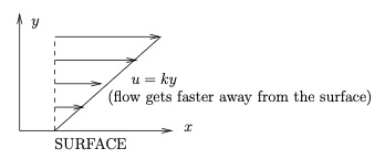
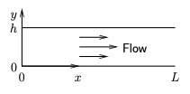
\begin{equation*} 0=-\pd{p}{x},\quad0=-\pd{p}{y},\quad0=-\pd{p}{z}, \end{equation*}

and thus \(p\) is constant everywhere in space.

🔗

For a Newtonian fluid contained between parallel plates moving tangentially, we obtain a shear flow in the gap. The velocity varies linearly across the gap and matches the plate velocity at each of the two plates. This is called Couette flow and it is an exact solution of the Navier–Stokes and continuity equations:

\(\rho\partial\bu/\partial t\text{:}\) The flow is steady so this term is zero.
🔗

🔗
\(\rho\bu\cdot\nabla\bu\text{:}\) Since \(\bu\) is directed tangential to the plates, \(\bu\cdot\nabla\) is a derivative in the tangential direction; however, \(\bu\) varies only in the direction normal to the plates. Therefore, \(\bu\cdot\nabla\bu\) is zero for this flow.
🔗

🔗
\(-\nabla p\text{:}\) The pressure is uniform, so this term is zero.
🔗

🔗
\(\mu\nabla^2\bu\text{:}\) The flow has a linear profile so \(\nabla^2\bu\) is zero.
🔗

🔗
\(\nabla\cdot\bu\text{:}\) The flow only varies in the direction normal to the plates and the normal component of the velocity is zero, meaning that this term is zero.
🔗

🔗

🔗

Figure 7.8.3. Shear flow would be generated under the block.
🔗

🔗

Example 7.8.4. Hagen–Poiseuille flow (or Poiseuille flow).

Poiseuille flow is the characteristic flow seen when an incompressible Newtonian fluid flows steadily along a cylindrical pipe whose length is long compared with its diameter. To find the fluid velocity we use cylindrical polar coordinates \((r,\theta,z)\text{,}\) and assume that the pipe wall is at \(r=a\text{.}\) We denote the fluid velocity components as \((u,v,w)\) in the three coordinate directions, i.e. \(\bu=u\hat{\br}+v\hat{\btheta}+w\hat{\bz}\text{,}\) and assume a no-slip boundary condition at the pipe wall:

\begin{equation} u=v=w=0\quad\mathrm{at}\quad r=a.\tag{7.8.1} \end{equation}

We also assume that the flow is steady, is axisymmetric, has no swirl (i.e.no azimuthal flow), is fully-developed, and we neglect gravity.

Steady flow:

\begin{equation*} \pd{u}{t}=\pd{v}{t}=\pd{w}{t}=\pd{p}{t}=0; \end{equation*}

🔗

🔗
Axisymmetric flow:

\begin{equation*} \pd{u}{\theta}=\pd{v}{\theta}=\pd{w}{\theta}=\pd{p}{\theta}=0; \end{equation*}

🔗

🔗
No swirl:

\begin{equation*} v=0; \end{equation*}

🔗

🔗
Fully-developed flow means the fluid velocity doesn’t change as we move along the pipe (we ignore end effects since the pipe length is long compared to the diameter), and also that the axial pressure gradient is constant, i.e.

\begin{align*} &\pd{u}{z}=\pd{v}{z}=\pd{w}{z}=0\\ &\pd{p}{z}=-G\mathrm{(constant)}. \end{align*}

🔗

🔗

🔗

Since the fluid is incompressible and Newtonian we take as our starting point the Navier–Stokes and continuity equations in cylindrical polar coordinates Remark 7.5.11. The continuity equation is

\begin{equation*} \bnabla\cdot\bu=\frac1r\pd{(ru)}{r}+\frac1r\pd{v}{\theta}+\pd{w}{z}=0, \end{equation*}

and applying assumptions 2 (or 3) and 4 in the list above, we get

\begin{equation*} \frac1r\pd{(ru)}{r}=0 \quad\Rightarrow\quad u=\frac Ar, \end{equation*}

where \(A\) is constant. Applying the boundary conditions (7.8.1) gives \(A=0\text{,}\) and therefore \(u=0\text{,}\) so the velocity is axial \(\bu=(0,0,w)=w\hat{\bz}\text{.}\)

🔗

Neglecting time-dependence and gravity, the Navier–Stokes equations (7.5.1) are:

\begin{equation} \rho\left(\bu\cdot\bnabla\right)\bu=-\bnabla p+\mu\nabla^2\bu.\tag{7.8.2} \end{equation}

We take the terms individually:

Since \(\bu=w\hat{\bz}\text{,}\)

\begin{equation*} \bu\cdot\bnabla=w\pd{}{z} \quad\Rightarrow\quad \left(\bu\cdot\bnabla\right)\bu =w\pd{(w\hat{\bz})}{z}, \end{equation*}

and this equals zero by the fully developed assumption (4 above).

🔗

🔗
The pressure gradient equals

\begin{equation*} \bnabla p=\pd{p}{r}\hat{\br}-G\hat{\bz}. \end{equation*}

🔗

🔗
Since the \(\theta\)- and \(z\)-derivatives of \(w\) vanish,

\begin{equation*} \nabla^2\bu =\nabla^2\left(w\hat{\bz}\right) =\left(\nabla^2w\right)\hat{\bz} =\frac1r\pd{}{r}\left(r\pd{w}{r}\right)\hat{\bz}. \end{equation*}

Note that the formula used here for \(\nabla^2w\) is standard and can be looked up (so you don’t need to remember it, though you should be aware that the gradient operator \(\bnabla\) takes a different form in polar coordinates).

🔗

🔗

Thus the three components of the Navier–Stokes equation (7.8.2) are

\(r\)-component:

\begin{equation*} 0=-\pd{p}{r}. \end{equation*}

🔗

🔗
\(\theta\)-component:

\begin{equation*} 0=0. \end{equation*}

🔗

🔗
\(z\)-component:

\begin{equation*} 0=G+\frac{\mu}{r}\pd{}{r}\left(r\pd{w}{r}\right). \end{equation*}

🔗

🔗

Solving the \(z\)-component gives the axial velocity component \(w\text{:}\)

\begin{align*} &\pd{}{r}\left(r\pd{w}{r}\right)=0-\frac{G}{\mu}r\\ \Rightarrow\quad& r\pd{w}{r}=-\frac{Gr^2}{2\mu}+A\\ \Rightarrow\quad& \pd{w}{r}=-\frac{Gr}{2\mu}+\frac{A}{r}\\ \Rightarrow\quad& w=-\frac{Gr^2}{4\mu}+A\ln r+B. \end{align*}

We require \(A=0\) for regularity of the solution at \(r=0\text{,}\) and since the boundary condition (7.8.1) has \(w=0\) at \(r=a\text{,}\) we must set \(B=Ga^2/(4\mu)\text{.}\) Therefore the fluid velocity in Poiseuille flow is given by

\begin{equation} u=v=0\quad w=\frac{G}{4\mu}\left(a^2-r^2\right),\tag{7.8.3} \end{equation}

which is illustrated in Figure 7.8.5.

🔗

Figure 7.8.5. Sketch of Poiseuille flow velocity profile.
🔗

The celebrated Hagen–Poiseuille formula can be derived from (7.8.3):

\begin{equation} \Delta P=\frac{8\mu LQ}{\pi a^4}.\tag{7.8.4} \end{equation}

This relates the volumetric flux \(Q\) and pressure drop \(\Delta P\) along a circular pipe of length \(L\) and radius \(a\) in a Newtonian fluid with shear viscosity \(\mu\) for steady, fully developed flow. You will derive this result in Exercise 7.9.12.

🔗

We now consider two generalisations:

Womersley flow: This is pipe flow driven by an axial pressure drop along the pipe that oscillates sinusoidally in time (Poiseuille flow was driven by a constant pressure gradient). Unlike Poiseuille flow, the exact profile of the flow depends on a parameter called the Womersley parameter (which depends on the frequency). Figure 7.8.6 shows an example. The flow is:
- Unidirectional axial flow (purely along the pipe)
  🔗
  
  🔗
- Axisymmetric
  🔗
  
  🔗
- Flow direction oscillates in time. Sometimes the flow goes in both directions at once, which can be seen in Figure 7.8.6.
  🔗
  
  🔗
If we add the velocity field of Poiseuille flow (7.8.3) onto the Womersley flow velocity field, we obtain the flow that would be driven by a pressure gradient that oscillates about a non-zero mean. Flow profiles of this sort can be seen in blood flow, since the beating of the heart provides a pressure gradient that can be approximated by a constant plus sinusoidally varying component.

🔗
🔗
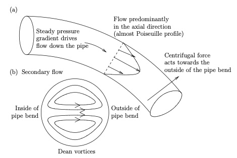
Dean flow: This is a steady flow driven by a steady prescribed pressure drop along the pipe, but the pipe is curved, see Figure 7.8.7. Within the pipe the flow is predominantly in the axial direction, but the centrifugal force due to the curvature drives a secondary flow across the centre of the pipe towards the outside of the bend, and then back around the walls of the pipe towards the inside of the bend. This secondary flow forms Dean vortices. This is thought to provide a possible explanation as to why the disease atherosclerosis in arteries is more common on the inside of bends in arteries, since the cells lining the artery walls are more healthy in conditions of high stress. Figure 7.8.7 shows shows the secondary flow in the transverse cross section, which are termed Dean vortices.
🔗

🔗

🔗

Figure 7.8.6. Sketch of Womersley flow velocity profile.
🔗

Figure 7.8.7. Sketch of Dean flow velocity profile: (a) longitudinal cross-section; (b) transverse cross-section.
🔗

🔗

Example 7.8.8. Channel flow.

This is the characteristic flow seen between two fixed parallel plates driven by a steady pressure gradient. The assumptions are:

Parallel fixed plates
🔗

🔗
Two-dimensional flow
🔗

🔗
Steady flow
🔗

🔗
Fully developed flow
🔗

🔗

The resulting profile is shown in Figure 7.8.9. The flow is parabolic and looks similar to a cross-section of Poiseuille flow. See also the cartoon of channel flow between two plates.

🔗

Figure 7.8.9. Sketch of channel flow velocity profile.
🔗

🔗

Example 7.8.10. Axisymmetric Couette flow.

This is the characteristic flow that is observed between cylinders that are rotating relative to one another. We assume:

Coaxial cylinders, rotating at different constant angular velocities
🔗

🔗
Two-dimensional flow (no dependence on \(z\)-coordinate)
🔗

🔗
Axisymmetric flow
🔗

🔗
Steady flow
🔗

🔗

The resulting flow is illustrated in Figure 7.8.11.

🔗

Figure 7.8.11. Sketch of axisymmetric Couette flow.
🔗

🔗

Example 7.8.12. Stokes boundary layer.

Figure 7.8.13. Sketch of set up for Stokes boundary layer.
🔗

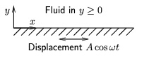
In this question you will investigate the flow field generated next to a flat oscillating plate. Assume that the plate is at \(y=0\) with an incompressible Newtonian fluid of density \(\rho\) and kinematic viscosity \(\nu\) in \(y>0\text{,}\) and that the plate oscillates purely in the \(x\)-direction with displacement \(A\cos\omega t\,\bi\) at time \(t\text{,}\) as shown in Figure 7.8.13. You may also assume that the plate and volume of fluid are large enough that you can neglect their boundaries (that is, the plate occupies the whole plane \(y=0\) and the fluid occupies the whole of \(y>0\)) and that the plate has been oscillating long enough so that the whole fluid is oscillating periodically.

🔗

(a)

Write down the equations and boundary conditions governing the flow.

🔗

Solution.

The fluid is governed by the Navier–Stokes and continuity equations:

\begin{equation*} \pd{\bu}{t}+\bu\cdot\bnabla\bu=-\frac1{\rho}\bnabla p+\nu\nabla^2\bu,\quad \bnabla\cdot\bu=0. \end{equation*}

At \(y=0\) the boundary conditions are

\begin{equation*} u=-A\omega\sin\omega t,\quad v=w=0. \end{equation*}

🔗

(b)

Write down assumptions about the components of the fluid flow and their dependence on the spatial coordinates \(x\text{,}\) \(y\) and \(z\text{.}\) Use this to simplify the the governing equations and boundary conditions.

🔗

Solution.

We assume this is a two-dimensional flow, with \(w=0\) and all components not depending on \(z\text{.}\) In addition we assume the velocity components do not depend on \(x\) (because translating the problem in the \(x\)-direction is the same problem). Thus we have \(u(y,t)\text{,}\) \(v(y,t)\text{,}\) \(w=0\) and \(p(y,t)\text{.}\)

🔗

The continuity equation is

\begin{equation*} \pd{u}{x}+\pd{v}{y}+\pd{w}{z}=0. \end{equation*}

The first and third terms are zero by assumption, and therefore

\begin{equation*} \pd{v}{y}=0. \end{equation*}

Hence \(v\) is constant, and the boundary condition \(v=0\) at \(y=0\) implies that \(v=0\) everywhere. The three components of the Navier–Stokes equation simplify to

\begin{align*} &\pd{u}{t}+0+0+0=0+\nu\left(0+\pd{^2u}{y^2}+0\right),\\\\ &0+0+0+0=-\frac1{\rho}\pd{p}{y}+\nu\left(0+0+0\right),\\\\ &0+0+0+0=0+\nu\left(0+0+0\right). \end{align*}

Thus \(p\) is constant in space and the only non-trivial equation is

\begin{equation*} \pd{u}{t}=\nu\pd{^2u}{y^2}, \end{equation*}

together with boundary conditions \(u=-A\omega\sin\omega t\) at \(y=0\text{.}\)

🔗

(c)

Make the assumption that the flow and pressure are sinusoidal, that is \(\bu(\bx,t)=\bu(\bx)e^{\im\omega t}+\overline{\bu(\bx)}e^{-\im\omega t}\) and \(p(\bx,t)=P(\bx)e^{\im\omega t}+\overline{P(\bx)}e^{-\im\omega t}\text{.}\) Use this to simplify and solve the governing equations to find the velocity field.

🔗

Solution.

The periodic assumption simplifies to \(u=U(y)e^{\im\omega t}+\overline{U(y)}e^{-\im\omega t}\) (the other components are not needed). Substituting into the governing equation,

\begin{equation*} \im\omega Ue^{i\omega t}-\im\omega \overline{U(y)}e^{-\im\omega t} =\nu\left(\frac{d^2U}{dy^2}e^{\im\omega t} +\frac{d^2\overline{U}}{dy^2}e^{-\im\omega t}\right). \end{equation*}

The coefficients of \(e^{\im\omega t}\) must balance and the coefficients of \(e^{-\im\omega t}\) must balance. Therefore

\begin{equation*} \im\omega U=\nu\frac{d^2U}{dy^2}, \quad\mathrm{and}\quad -\im\omega\overline{U}=\nu\frac{d^2\overline{U}}{dy^2}. \end{equation*}

These two equations are the complex conjugates of one another, so we only need to solve one of them, which gives the general solution

\begin{equation*} U=C_1e^{\sqrt{\frac{\im\omega}{\nu}}y}+C_2e^{-\sqrt{\frac{\im\omega}{\nu}}y}. \end{equation*}

The function \(e^{\sqrt{\frac{\im\omega}{\nu}}y}\rightarrow\infty\) as \(y\rightarrow\infty\text{,}\) and thus \(C_1=0\text{.}\) The boundary condition \(u=-A\omega\sin\omega t =(A\omega i/2)e^{\im\omega t}-(A\omega\im/2)e^{-\im\omega t}\) at \(y=0\text{.}\) Hence \(U=A\omega\im/2\text{,}\) meaning that \(C_2=A\omega\im/2\text{.}\) Hence

\begin{align*} u=&\frac{A\omega \im}{2}e^{-\sqrt{\frac{\im\omega}{\nu}}y+\im\omega t}-\frac{A\omega \im}{2}e^{-\sqrt{\frac{-\im\omega}{\nu}}y-\im\omega t}\\\\ =&-\frac{A\omega}{2\im}\left(e^{-(1+\im)\sqrt{\frac{\omega}{2\nu}}y+\im\omega t}-e^{-(1-\im)\sqrt{\frac{\omega}{2\nu}}y-\im\omega t}\right)\\\\ =&-A\omega e^{-\sqrt{\frac{\omega}{2\nu}}y}\frac{\left(e^{\im(-\sqrt{\frac{\omega}{2\nu}}y+\omega t)}-e^{-\im(-\sqrt{\frac{\omega}{2\nu}}y+\omega t)}\right)}{2\im}\\\\ =&-A\omega e^{-\sqrt{\frac{\omega}{2\nu}}y}\sin\left(\omega t-\sqrt{\frac{\omega}{2\nu}}y\right). \end{align*}

🔗

(d)

Sketch the velocity profile at time \(t\text{.}\)

🔗

Solution.

The velocity profile is a sinusoidal function whose amplitude decays exponentially with the distance from the surface.

🔗

Figure 7.8.14. Stokes boundary layer flow.
🔗

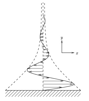
This is a famous exact solution of the Navier–Stokes equations, and the flow we have found here is characteristic of the flow that exists near an oscillating boundary. Note that the flow decays away from the wall, and for this reason it is often described as a boundary later, and the solution is called Stokes boundary layer flow.

🔗

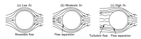
Example 7.8.15. Low-Reynolds-number flow past a sphere (non-examinable).

This section is non-examinable.

🔗

Figure 7.8.16. Photographs of a sphere moving through a fluid with \(\mathrm{Re} = 0.1\text{.}\) The top photograph is in the reference frame in which the sphere is stationary, and the bottom photograph is in a fixed frame, (note the shadow cast by the sphere is not indicative of the flow). Taken from [3], and see also Figs. 25, 51, 56, 58 from this book, which show the flow for higher Reynolds numbers.
🔗

Figure 7.8.17. Sketches of the flow field around of a fixed sphere in a moving fluid for (a) low, (b) moderate and (c) high Reynolds numbers.
🔗

In this section we find the flow around a sphere moving through a fluid at a low Reynolds number, using a Stokes streamfunction. We use this to find the drag on the sphere. Figure 7.8.16 shows two photographs of the same flow, but visualised in two different ways, and Figure 7.8.17 shows sketches of the flow for a range of Reynolds numbers.

🔗

The calculation shows that the drag force experienced by an object moving through a fluid at low Reynolds numbers can be derived from the Stokes equations. This analysis shows that the Stokes drag on a sphere is \(6\pi\mu Ua\) in the direction opposing motion, which holds as long as \(\rho Ua/\mu\ll1\text{.}\) This is a famous classical result in fluid mechanics.

🔗

This principle is used in a falling ball viscometer in which a small spherical ball of known radius \(a\) and mass \(m\) is dropped into a fluid, whose viscosity \(\mu\) we wish to measure. Once the ball has reached its terminal falling velocity \(U\text{,}\) the forces on it must be in equilibrium, meaning that the force of gravity balances the drag force. Assuming the sphere is small enough and going slowly enough and the fluid is viscous enough that the flow has a low Reynolds number, the drag is given by \(6\pi\mu Ua\) and the force of gravity is \(mg\text{,}\) where \(g\) is the acceleration due to gravity. Thus

\begin{equation*} \mu=\frac{mg}{6\pi Ua}, \end{equation*}

and so measuring the terminal velocity and substituting into this equation gives an estimate of the viscosity of the fluid.

🔗

We assume the flow is axisymmetric and work in a moving reference frame centred on the sphere using spherical coordinates. As shown in Subsection 6.3.1, we can write the velocity in terms of a Stokes streamfunction \(\Psi\) using (6.3.1):

\begin{align*} u_r=&\frac1{r^2\sin\theta}\pd{\Psi}{\theta},\\ u_\theta=&-\frac1{r\sin\theta}\pd{\Psi}{r},\\ u_\phi=&0. \end{align*}

From (6.3.8), the vorticity is given by

\begin{equation*} \bomega=-\frac1{r\sin\theta}\left(\mathcal{L}_s\left(\Psi\right)\right)\hat\bphi, \end{equation*}

where the differential operator \(L_s\) is a variant of the Laplacian operator, defined by its action on a function \(A\) by

\begin{equation} \mathcal{L}_s\left(A\right)=\pd{^2A}{r^2} +\frac{\sin\theta}{r^2}\pd{}{\theta}\left(\frac1{\sin\theta}\pd{A}{\theta}\right).\tag{7.8.5} \end{equation}

At low Reynolds numbers, we take the curl of the Stokes equation (7.5.4) to give

\begin{equation*} \nabla^2\bomega=\bzero, \end{equation*}

and, after some work, we may show this is equivalent to

\begin{equation} \mathcal{L}_s^2\Psi=0.\tag{7.8.6} \end{equation}

We need boundary conditions on \(\Psi\text{,}\) which are given by the following:

No-slip conditions on the surface of the sphere (\(r=a\)). Using the expressions for \(u_r\) and \(u_\theta\) above, these become

\begin{align*} &u_r=0\quad\Rightarrow\quad\pd{\Psi}{\theta}=0,\\ &u_\theta=0\quad\Rightarrow\quad\pd{\Psi}{r}=0. \end{align*}

🔗

🔗
As \(r\rightarrow\infty\) we must have uniform flow with velocity \(U\) in the direction \(\theta=\pi\text{.}\) Using the expressions for the velocity components \(u_r\) and \(u_\theta\) above, these become

\begin{align*} &u_r\sim -U\cos\theta\quad\Rightarrow\quad \pd{\Psi}{\theta}\sim-Ur^2\sin\theta\cos\theta,\\ &u_\theta\sim U\sin\theta\quad\Rightarrow\quad \pd{\Psi}{r}\sim-Ur\sin^2\theta. \end{align*}

Combining these we get

\begin{equation*} \Psi\sim-\frac12Ur^2\sin^2\theta+C, \end{equation*}

where \(C\) is constant. Adding a constant onto the streamfunction does not affect the velocity, and thus we may arbitrarily set \(C=0\text{,}\) giving

\begin{equation} \Psi\sim-\frac12Ur^2\sin^2\theta\quad\mathrm{as}\quad r\rightarrow\infty.\tag{7.8.7} \end{equation}

🔗

🔗

Thus we have to solve (7.8.6) subject to the \(\partial\Psi/\partial r=\partial\Psi/\partial\theta=0\) on \(r=a\) and (7.8.7) as \(r\rightarrow\infty\text{.}\) We try a separable function

\begin{equation} \Psi=f(r)g(\theta),\tag{7.8.8} \end{equation}

and the condition (7.8.7) implies that \(g(\theta)=\sin^2\theta\) (or a multiple thereof). Substituting (7.8.8) into (7.8.6) and using (7.8.5), after some algebra we obtain

\begin{equation} \dd{^4f}{r^4} -\frac{4}{r^2}\dd{^2f}{r^2} +\frac{8}{r^3}\dd{f}{r} -\frac{8f}{r^4} =0.\tag{7.8.9} \end{equation}

We try \(f\propto r^\alpha\) and obtain

\begin{align*} &\alpha(\alpha-1)(\alpha-2)(\alpha-3)r^{\alpha-4} -\frac{4}{r^2}\alpha(\alpha-1)r^{\alpha-2} +\frac{8}{r^3}\alpha r^{\alpha-1}-\frac{8}{r^4}r^\alpha=0\\ \Rightarrow\quad &\alpha(\alpha-1)(\alpha-2)(\alpha-3)-4\alpha(\alpha-1)+8\alpha-8=0\\ \Rightarrow\quad &(\alpha-4)(\alpha-2)(\alpha+1)(\alpha-1)=0. \end{align*}

Thus \(\alpha=4,2,1\) or \(-1\text{,}\) and so the general solution of (7.8.9) is

\begin{equation*} f(r)=C_1r^4+C_2r^2+C_3r+\frac{C_4}{r}. \end{equation*}

Enforcing the behaviour (7.8.7) as \(r\rightarrow\infty\text{,}\) we need \(f\sim-Ur^2/2\text{,}\) and so \(C_1=0\text{,}\) \(C_2=-U/2\text{.}\) Thus

\begin{equation*} f(r)=-\frac12Ur^2+C_3r+\frac{C_4}{r}. \end{equation*}

🔗

🔗
Applying the boundary condition \(\partial\Psi/\partial\theta=0\) at \(r=a\text{,}\)

\begin{align*} &\left.\pd{\Psi}{\theta}\right|_{r=a}=0\\ \Rightarrow\quad&f(a)g'(\theta)=0\\ \Rightarrow\quad&\left(-\frac12Ua^2+C_3a+\frac{C_4}{a}\right) \left(2\sin\theta\cos\theta\right)=0 \end{align*}

which must be true for all values of \(\theta\text{.}\) Thus

\begin{equation} -\frac12Ua^2+C_3a+\frac{C_4}{a}=0.\tag{7.8.10} \end{equation}

🔗

🔗
Applying the boundary condition \(\partial\Psi/\partial r=0\) at \(r=a\text{,}\)

\begin{align*} &\left.\pd{\Psi}{r}\right|_{r=a}=0\\ \Rightarrow\quad&f'(a)g(\theta)=0\\ \Rightarrow\quad&\left(-Ua+C_3-\frac{C_4}{a^2}\right)\left(\sin^2\theta\right)=0, \end{align*}

which must be true for all \(\theta\text{.}\) Thus

\begin{equation} -Ua+C_3-\frac{C_4}{a^2}=0.\tag{7.8.11} \end{equation}

🔗

🔗

Equations (7.8.10) and (7.8.11) have the solution \(C_3=3Ua/4\) and \(C_4=-Ua^3/4\text{.}\) Thus

\begin{equation*} \Psi=-\frac{U}{4r}\left(a^3-3ar^2+2r^3\right)\sin^2\theta, \end{equation*}

and we can substitute this into the expressions for the components of the velocity field to obtain the velocity:

\begin{align*} &u_r=\frac1{r^2\sin\theta}\pd{\Psi}{\theta} =-\frac{U}{2}\left(2-\frac{3a}{r}+\frac{a^3}{r^3}\right)\cos\theta =-\frac{U}{2}\left(1-\frac{a}{r}\right)^2\left(2+\frac{a}{r}\right)\cos\theta,\\ &u_\theta=-\frac1{r\sin\theta}\pd{\Psi}{r} =\frac{U}{4}\left(4-\frac{3a}{r}-\frac{a^3}{r^3}\right)\sin\theta =\frac{U}{4}\left(1-\frac{a}{r}\right)\left(4+\frac{a}{r}+\frac{a^2}{r^2}\right)\sin\theta,\\ &u_\phi=0. \end{align*}

🔗

We can also find the pressure using the Stokes equation in the form \(\bnabla p=\mu\nabla^2\bu\text{.}\) After a lot of algebra we obtain

\begin{equation*} \pd{p}{r}=-\frac{3\mu Ua}{r^3}\cos\theta,\quad \frac1r\pd{p}{\theta}=-\frac{3\mu Ua}{2r^3}\sin\theta,\quad \frac1{r\sin\theta}\pd{p}{\phi}=0, \end{equation*}

which we solve to find

\begin{equation*} p=p_0+\frac{3\mu Ua}{2r^2}\cos\theta, \end{equation*}

where \(p_0\) is constant.

🔗

Perhaps the most interesting application of this solution is to find the drag on the sphere, which is the total force of the fluid on the sphere, retarding the motion. Since the stress is the force per unit area on the sphere, the drag equals the integral of the stress over the surface. We find the stress using

\begin{equation} \btau=\bsigma\hat\br,\quad\mathrm{where}\quad \bsigma=-p \bI +2\mu \be\quad\mathrm{and}\quad \hat\br=\left(\begin{array}{c}1\\0\\0\end{array}\right).\tag{7.8.12} \end{equation}

We use the expression for \(\be\) in spherical polar coordinates (7.4.8), and then (7.8.12) gives the stress on the surface as

\begin{align*} \btau=&\left.\left(\begin{array}{c} -p+2\mu\pd{u_r}{r}\\ \mu\left(r\pd{(u_\theta/r)}{r}+\frac1r\pd{u_r}{\theta}\right)\\ \mu\left(\pd{(u_\phi/r)}{r}+\frac1{r\sin\theta}\pd{u_r}{\phi}\right) \end{array}\right)\right|_{r=a}\\ =&\left.\left(-p+2\mu\pd{u_r}{r}\right)\right|_{r=a}\hat\br +\left.\mu\left(r\pd{(u_\theta/r)}{r}+\frac1r\pd{u_r}{\theta}\right)\right|_{r=a}\hat\btheta\\ &+\left.\mu\left(\pd{(u_\phi/r)}{r}+\frac1{r\sin\theta}\pd{u_r}{\phi}\right)\right|_{r=a}\hat\bphi. \end{align*}

On substituting in the expressions for the velocity components \(u_r\text{,}\) \(u_\theta\text{,}\) \(u_\phi\text{,}\) we find that

\begin{equation*} \btau =\left(-p_0-\frac{3\mu U}{2a}\cos\theta\right)\hat\br+\frac{3\mu U}{2a}\sin\theta\hat\btheta+0\hat\bphi =-p_0\hat\br+\frac{3\mu U}{2a}\left(\sin\theta\hat\btheta-\cos\theta\hat\br\right).\label{eq:tauworking} \end{equation*}

We express the bracket \((\sin\theta\hat\btheta-\cos\theta\hat\br)\) in this equation in terms of Cartesian coordinates, using the conversion formulae

\begin{equation*} \hat\br=\cos\phi\sin\theta\bI+\sin\phi\sin\theta\bj+\cos\theta\bk,\quad \hat\btheta=\cos\phi\cos\theta\bI+\sin\phi\cos\theta\bj-\sin\theta\bk. \end{equation*}

Substituting this into the expression for \(\btau\text{,}\) we obtain the stress

\begin{equation*} \btau=-p_0\hat\br-\frac{3\mu U}{2a}\bk. \end{equation*}

The drag equals the integral of \(\btau\) over the surface of the sphere. The integral of the term \(-p_0\hat\br\) is zero because this force cancels on opposite sides of the sphere, but the term \(-\frac{3\mu U}{2a}\hat\bk\) is always in the same direction; thus the total drag force is this term times the area, which is

\begin{equation*} \left(-\frac{3\mu U}{2a}\hat\bk\right)\times\left(4\pi a^2\right)=-6\pi\mu Ua\hat\bk. \end{equation*}

Thus the drag force is \(\boxed{6\pi\mu Ua}\) in the direction opposing motion. This is called the Stokes drag and it is a famous result in fluid mechanics.

🔗

Remark 7.8.18.

This derivation is extremely complicated in terms of the algebra, and you would certainly not be asked to reproduce something so long-winded as this in this course. However, you should understand the concepts, and be able to follow the general argument. In fact the mathematics presented here is very elegant indeed, and it is amazing that an exact solution exists and can be calculated.

🔗

Remark 7.8.19.

Notice that in the course of the derivation (7.8.8), we made the assumption that \(\Psi\) is separable. Thus we have not rigorously shown that the solution we found was unique, that is there might be other solutions to this problem that satisfy the boundary conditions at \(r=a\) and the condition as \(r\rightarrow\infty\text{.}\)

🔗

Remark 7.8.20.

This solution is the same as the irrotational flow solution (see Subsection 6.3.3). Note that for any real fluid (i.e. one with viscosity), this solution would only be seen for low Reynolds numbers, despite the fact that inviscid fluids correspond to high Reynolds numbers.

🔗

Example 7.8.21. Womersley flow (non-examinable).

This section is non-examinable.

🔗

Womersley flow occurs in pipes in which there is an imposed oscillating pressure gradient. Characteristics of this flow are often seen in blood flow in arteries, since the flow and pressure gradient are unsteady. As for the derivation of Poiseuille flow, we consider a long, circular cylindrical pipe of radius \(a\text{,}\) and work in cylindrical polar coordinates centred on the axis of the pipe. We make the following assumptions:

The flow is fully developed; thus \(\partial\bu/\partial z=0\text{.}\)
🔗

🔗
The flow is axisymmetric; thus \(\partial\bu/\partial\theta=\partial p/\partial\theta=0\text{.}\)
🔗

🔗
The flow has a symmetry in a diameter of the cross-section. In turn this means there is no swirl in the flow, and thus \(u_\theta=0\text{.}\)
🔗

🔗

The derivation proceed similarly to that of Poiseuille flow (so we cover it quite briefly here). With the assumptions, the continuity equation reduces to

\begin{equation*} \frac1r\pd{}{r}\left(ru_r\right)=0, \end{equation*}

which gives \(u_r\propto1/r\text{,}\) whereupon the boundary condition implies that the constant of proportionality is zero, and hence \(u_r=0\text{.}\) Thus the only flow component is the axial flow, \(u_z\text{,}\) which, according to the assumptions, is a function of \(r\) and \(t\) only (and does not depend on either \(\theta\) or \(z\)). The radial and azimuthal components of the Navier–Stokes equation reduce to the equations

\begin{equation*} \pd{p}{r}=\pd{p}{\theta}=0, \end{equation*}

and thus \(p\) is a function of \(z\) and \(t\) only. The axial component of the Navier–Stokes equation is

\begin{equation} \rho\pd{u_z}{t}=-\pd{p}{z}+\mu\frac1r\pd{}{r}\left(r\pd{u_z}{r}\right).\tag{7.8.13} \end{equation}

Consider what happens to the three terms in this equation at fixed values of \(t\) and \(r\) as \(z\) alone is varied. Since \(u_z\) is not a function of \(z\text{,}\) the only term that can vary is \(\pd{p}{z}\text{,}\) while the other two terms stay constant. Since equality must be maintained this shows that, in fact, \(\pd{p}{z}\) must be fixed as \(z\) varies, and thus \(p=A(t)z+B(t)\text{,}\) where \(A\) and \(B\) are unknown functions of time. We set \(G(t)=-A(t)\) to be the pressure gradient of the flow at time \(t\text{.}\)

🔗

In Poiseuille flow \(G\) is fixed in time, but in Womersley flow we set \(G(t)=G_0\cos\omega t\text{,}\) where \(G_0\) is constant (by fixing the origin of time we may fix \(G_0\) to be real and positive). We can write this as

\begin{equation*} G(t)=\frac{G_0}{2}e^{\im\omega t}+\mathrm{c.c.}, \end{equation*}

where \(\mathrm{c.c.}\) denotes the complex conjugate. We try a solution of the form

\begin{equation} u_z(r,t)=U(r)e^{\im\omega t}+\mathrm{c.c.},\label{eq:udecomp}\tag{7.8.14} \end{equation}

where \(U\) is a complex-valued function, and, substituting this into (7.8.13), we obtain

\begin{align*} &\rho\im\omega Ue^{\im\omega t}-\rho\im\omega\overline{U}e^{-\im\omega t} =\frac{G_0}2e^{\im\omega t}+\frac{G_0}2e^{-\im\omega t} +\mu\frac1r\pd{}{r}\left(r\pd{U}{r}\right)e^{\im\omega t}+\mu\frac1r\pd{}{r}\left(r\pd{\overline{U}}{r}\right)e^{-\im\omega t}\\ \Rightarrow\quad& \left\{\rho\im\omega U-\frac{G_0}2-\mu\frac1r\pd{}{r}\left(r\pd{U}{r}\right)\right\}e^{\im\omega t} +\left\{-\rho\im\omega\overline{U}-\frac{G_0}2-\mu\frac1r\pd{}{r}\left(r\pd{\overline{U}}{r}\right)\right\}e^{-\im\omega t} =0. \end{align*}

This equation must be true for all values of \(t\text{,}\) which means that both of the expressions in brackets \(\{\}\) must be be zero. Since the two bracketed expressions are complex conjugates of one another, we only need to consider the first bracket. Thus

\begin{equation*} \im\omega\rho U-\frac{G_0}2-\mu\frac1r\dd{}{r}\left(r\dd{U}{r}\right)=0 \quad\Rightarrow\quad \dd{^2U}{r^2}+\frac1r\dd{U}{r}-\frac{\im\omega\rho}{\mu}U=-\frac{G_0}{2\mu}. \end{equation*}

This is a linear, second-order, non-constant-coefficient, non-homogeneous ordinary differential equation for \(U\text{.}\) We can therefore solve it as a complementary function \(U_{cf}\) plus a particular integral \(U_{pi}\text{.}\) The particular integral is given by

\begin{equation*} U_{pi}=\frac{G_0}{2\im\omega\rho}. \end{equation*}

To find the complementary function we must solve

\begin{equation*} \dd{^2U_{cf}}{r^2}+\frac1r\dd{U_{cf}}{r}-\frac{\im\omega\rho}{\mu}U_{cf}=0, \end{equation*}

and substituting \(s=(\sqrt{-\im\omega/\nu})r\) and simplifying, we remove the coefficients on the left-hand side to obtain

\begin{equation*} \dd{^2U_{cf}}{s^2}+\frac1s\dd{U_{cf}}{s}+U_{cf}=0. \end{equation*}

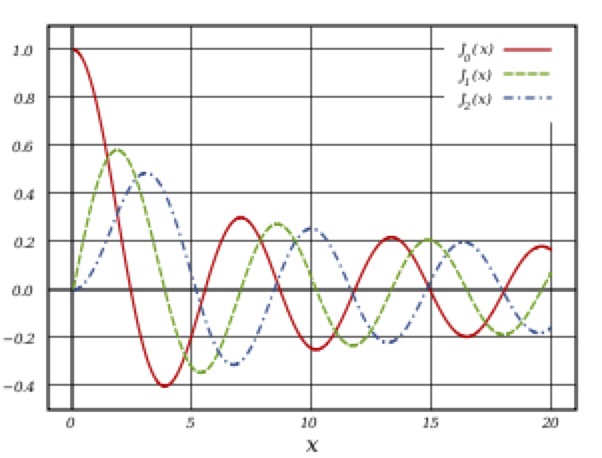
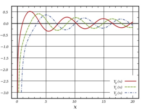
This equation is the standard form of a special equation called Bessel’s equation. The two linearly independent solutions are called Bessel functions of order zero, and they are denoted \(J_0\) and \(Y_0\text{,}\) see Figure 7.8.22 and Figure 7.8.23.

🔗

Figure 7.8.22. Bessel functions of the first kind \(J_0\text{,}\) \(J_1\) and \(J_2\) (from Wikipedia entry on Bessel functions).
🔗

Figure 7.8.23. Bessel functions of the second kind \(Y_0\text{,}\) \(Y_1\) and \(Y_2\) (from Wikipedia entry on Bessel functions).
🔗

We therefore obtain the complementary function

\begin{equation*} U_{cf}=C_1J_0(s)+C_2Y_0(s), \end{equation*}

where \(C_1\) and \(C_2\) are constants of integration, and thus

\begin{align*} U=U_{cf}+U_{pi} =&C_1J_0\left(\sqrt{\frac{-\im\omega}{\nu}}r\right)+C_2Y_0\left(\sqrt{\frac{-\im\omega}{\nu}}r\right)+\frac{G_0}{2\im\omega\rho}\\ =&C_1J_0\left(\sqrt{-\im}\alpha\frac{r}{a}\right)+C_2Y_0\left(\sqrt{-\im}\alpha\frac{r}{a}\right)+\frac{G_0}{2\im\omega\rho}, \end{align*}

where the Womersley number \(\alpha\) is a dimensionless parameter defined by

\begin{equation*} \alpha=\sqrt{\frac{\omega}{\nu}}. \end{equation*}

To find the constants \(C_1\) and \(C_2\) we apply the boundary conditions and regularity conditions at the origin \(r=0\) (as we did for Poiseuille flow):

At \(r=0\text{:}\) The function \(Y_0(x)\) tends to infinity as \(x\rightarrow0\) and so contributions from \(Y_0((\sqrt{-\im\omega/\nu})r)\) are not allowed, meaning that \(C_2\) must be set to zero.
🔗

🔗
At \(r=a\text{:}\) The no-slip boundary condition is \(u_z=0\) at the wall for all times, which from (7.8.14) means that \(U\) must also be zero at \(r=a\text{.}\) Substituting into the solution for \(U\) gives

\begin{equation*} C_1=-\frac{G_0}{2\im\omega\rho J_0(\sqrt{-\im}\alpha)}. \end{equation*}

🔗

🔗

Hence

\begin{equation*} U=\frac{G_0}{2\im\omega\rho}\left(1-\frac{J_0(\sqrt{-\im}\alpha r/a)}{J_0(\sqrt{-\im}\alpha)}\right), \end{equation*}

and, substituting this into (7.8.14), we get

\begin{equation} u_z=-\frac{\im G_0}{2\omega\rho}\left(1-\frac{J_0(\sqrt{-\im}\alpha r/a)}{J_0(\sqrt{-\im}\alpha)}\right)e^{\im\omega t}+\mathrm{c.c.}\label{eq:womersleyflow}\tag{7.8.15} \end{equation}

This is Womersley flow, which was first described by Womersley in 1955. The nondimensionalised flow profile is

\begin{equation*} u_z^*=-\frac{\im}{2}\left(1-\frac{J_0(\sqrt{-\im}\alpha r^*)}{J_0(\sqrt{-\im}\alpha)}\right)e^{\im t^*}+\mathrm{c.c.},\label{eq:womersleyflownondim} \end{equation*}

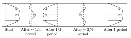
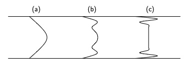
where \(u_z^*=u_z/(G_0/(\omega\rho))\text{,}\) \(r^*=r/a\text{,}\) \(t^*=\omega t\text{.}\) This nondimensionalisation shows that the flow is characterised by a single parameter, the Womersley number, \(\alpha\) (as opposed to 4 dimensional parameters: \(\rho\text{,}\) \(\mu\text{,}\) \(a\) and \(\omega\)). Sketches of the flow profiles for different values of \(\alpha\) are given in Figure~\ref{fig:womersley} and some movies will be shown in the lecture.

🔗

Figure 7.8.24. Snapshots of sketches of Womersley flow profiles for various Womersley numbers. (a) Low Womersley number (profile is Poiseuille flow multiplied by a time-dependent factor), (b) intermediate Womersley number, (c) high Womersley number (profile is flat across the interior with a boundary layer in which the flow oscillates rapidly).
🔗

Remark 7.8.25.

We may do a similar analysis for any prescribed periodic pressure gradient \(G(t)\text{.}\) To do this we decompose \(G(t)\) into a Fourier series sum of terms of different frequencies. We solve for the flow generated by each component of \(G(t)\) individually. The total flow is the sum of these flow components.

🔗

Remark 7.8.26.

In the human arterial system the Womersley number of the fundamental harmonic is different in different arteries and it takes values up to about 20.

🔗

Remark 7.8.27.

For small Womersley numbers we use the Taylor series expansion of the Bessel function:

\begin{equation*} J_0(z)=1-\frac{z^2}{4}+\dots \end{equation*}

to find an approximation of \(u_z\text{.}\)

\begin{align*} u_z=\frac{\im G_0}{2\omega\rho}\left(\frac{\im\alpha^2}4-\frac{\im}{4}\left(\frac{\alpha r}{a}\right)^2+\dots\right)e^{\im\omega t}+\mathrm{c.c.} \approx&-\frac{G_0}{8\mu}\left(a^2-r^2\right)e^{\im\omega t}+\mathrm{c.c.}\\ =&-\frac{G_0}{4\mu}\left(a^2-r^2\right)\cos\omega t, \end{align*}

which is a Poiseuille flow profile (multiplied by an oscillating amplitude). This flow is called quasi-steady, because this is the solution that we would obtain if we neglected the time-derivative term in the Navier–Stokes equation.

🔗

Remark 7.8.28.

For large Womersley numbers we use the standard asymptotic expansions for the Bessel function, which is:

\begin{equation*} J_0(z)\approx\sqrt{\frac{2}{\pi z}}\cos\left(z-\frac{\pi}{4}\right) \end{equation*}

when \(|z|\gg1\text{.}\) Letting \(z=x+\im y\text{,}\) where \(x\) and \(y\) are real, we can expand the cosine function:

\begin{equation*} J_0(z)\approx\sqrt{\frac{1}{2\pi z}}\left(e^{\im x-\im\pi/4}e^{-y}+e^{-\im x+\im\pi/4}e^{y}\right) \approx\sqrt{\frac{1}{2\pi z}}e^{\im x-\im\pi/4}e^{-y}=\sqrt{\frac{1}{2\pi z}}e^{\im z-\im\pi/4}. \end{equation*}

where the second approximation is valid if \(y\ll0\) (which is the case we have). Substituting into (7.8.15), we obtain

\begin{align*} u_z\approx&-\frac{\im G_0}{2\omega\rho}\left(1-\sqrt{\frac{a}{r}}e^{-\sqrt{\im}\alpha(1-r/a)}\right)e^{\im\omega t}+\mathrm{c.c.}\\ =&-\frac{\im G_0}{2\omega\rho}\left(1-\sqrt{\frac{a}{r}}e^{-\frac{\alpha}{\sqrt{2}}(1-\frac{r}{a})}e^{-\im\frac{\alpha}{\sqrt{2}}(1-\frac{r}{a})}\right)e^{\im\omega t}+\mathrm{c.c.} \end{align*}

Away from the boundaries, \(\frac{\alpha}{\sqrt{2}}(1-\frac{r}{a})\) is large and so the exponential terms in the bracket in this expression are very small, and

\begin{equation*} u_z\approx-\frac{\im G_0}{2\omega\rho}e^{\im\omega t}+\mathrm{c.c.} =\frac{G_0}{\omega\rho}\sin\omega t. \end{equation*}

This type of flow is called plug flow, since at any fixed time the profile is uniform across the interior.

🔗

Near the walls of the pipe the exponential terms become important. At the walls themselves, the flow is zero, and, as we move away, the expression for the velocity shows there are rapid oscillations that decrease in magnitude as we move away from the wall.

🔗

Thus we see that the flow is divided into two distinct regions. There is the core in which the dominant balance is between the pressure gradient and the inertial term (the time-derivative term), and in which the viscosity plays a minor role. Sometimes this is termed an inviscid core. The other region is the boundary layer, in which the viscosity is important. The width of the boundary layer is of the order of magnitude \(\alpha^{-1}a\) (often we would just say loosely that the boundary layer has width \(\alpha^{-1}a\)). Within a few \(\alpha^{-1}a\)’s away from the boundary, the flow is affected by the presence of the boundary, but further away the effect is negligible.

🔗

Another way that we could find the flow for large Womersley number is to use boundary layer analysis in the boundary, and an inviscid flow method (such as potential flow analysis) in the interior, and match the two solutions at the edge of the boundary layer. Since we have the exact solution valid for all Womersley numbers, this method of separating into the boundary layer and core regions is not necessary to find the solution. However, in many problems, no solution can be found in the general case, but a solution can be found in the particular case when one parameter is large or small. It is surprising how often such solutions are possible in real world problems, and this method often provides significant insight into the problem.

🔗

Prev Top Next