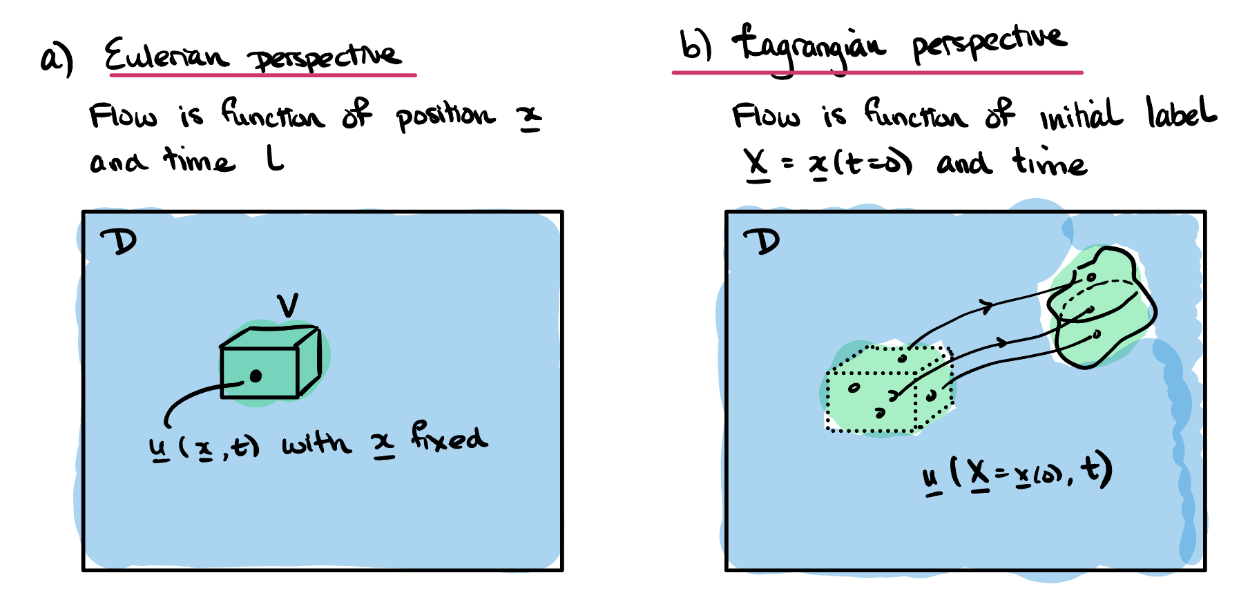
Eulerian and Lagrangian coordinates

Section 2.1 Eulerian and Lagrangian coordinates

There are essentially two natural ways to think of motion in a fluid. We can imagine positioning ourselves at a fixed point in space, $\bx = (x, y, z)\text{.}$ At this point, we then attempt to measure a fluid quantity such as the density, $\rho(\bx, t)\text{,}$ or temperature, $T(\bx, t)\text{.}$ This is essentially the Eulerian frame. One can imagine, for example, fixing sensor station into the ocean bottom, and obtaining measurements of the water temperature.

🔗

Figure 2.1.1. (a) The Eulerian interpretation; (b) the Lagrangian interpretation.
🔗

Alternatively, we can imagine tracking of a single fixed particle (or a fluid element) within the flow. The particle begins at some position. Let us define a label to describe the particle’s initial position. For example, if the particle’s position is given by

\begin{equation*} (x, y, z) = (x_1(t), y_1(t), z_1(t)), \end{equation*}

we can define the corresponding Lagrangian label as

\begin{equation*} \bX = (X, Y, Z) = (x_1(0), y_1(0), z_1(0)). \end{equation*}

We then ask for the corresponding measurement of the fluid quantity that corresponds to the label $\bX\text{.}$ For example, this is equivalent to tagging a free-floating buoy in the ocean with the label $\bX\text{,}$ then measuring the temperature of the water as the buoy drifts in the ocean. This Lagrangian temperature could be written $\mathcal{T}(\bX, t),$ where $\bX$ is simply a fixed quantity for the particular buoy.

🔗

We are now in a position to define the Eulerian velocity field of a fluid.

🔗

Definition 2.1.2.

The Eulerian velocity $\bu(\bx,t)$ is the velocity of the fluid at the point with spatial coordinates $\bx$ at time $t\text{.}$ Note that, in physical terms this velocity is the average velocity at the time $t$ of the fluid particles (e.g. molecules, ions) in a small box centred on the point $\bx\text{.}$ See also Remark 3.0.3 for a discussion of the continuum assumption.

🔗

It will be useful to introduce the concept of steady flow.

🔗

Definition 2.1.3.

A velocity field $\bu$ is defined as steady if it can be written $\bu=\bu(\bx)$ .

🔗

Note that steady flow does not mean that the fluid particles are not moving. It simply means that at a fixed point in space, the Eulerian velocity does not change in time. The Lagrangian velocity of a fluid particle will generally change in time, even in a steady flow.

🔗

A simple example of the conversion between the Eulerian and Lagrangian reference frames is in Exercise 2.3.3.

🔗

Subsection 2.1.1 The convective derivative

Let us now be more specific. We wish to consider how different quantities in our flow changes with time, but the matter is made complicated by the two above perspectives (fixed or following the flow).

🔗

Again, let us consider a scalar property of the fluid (for example, its density, temperature, velocity component, pressure, etc.), and let us suppose that this quantity is a function of both position, $\bx\text{,}$ and time, $t\text{,}$ and denote it by $f(\bx, t)\text{.}$ This is the Eulerian description of the property since it is defined by specifying a fixed position in space. Fixing $\bx$ and then measuring $f$ is akin to standing in the fluid at a fixed location and measuring the property value in time.

🔗

We can alternatively write the property by its Lagrangian description. That is, given a label $\bX\text{,}$ we obtain the current position of the particle associated with this label, $\bx(\bX, t)\text{,}$ then obtain its property value. This we can write as the following:

\begin{equation*} F(\bX, t) \equiv f(\bx(\bX, t), t). \end{equation*}

Now, fixing $\bX$ and changing $t$ corresponds to tracking the scalar property at a material point in the flow, or, equivalently, how $f$ changes as we move with the particle along the deforming fluid.

🔗

There are thus two ways of considering time derivatives.

🔗

Definition 2.1.4.

We use the normal partial derivative notation to refer to an Eulerian time derivative, considered at a fixed point in space:

\begin{equation*} \pd{}{t} \equiv \pd{}{t} \biggr\rvert_{\bx} = \text{rate of change with $\bx$ held constant}. \end{equation*}

🔗

On the other hand, the Lagrangian time derivative is defined at a fixed material point in the fluid.

\begin{equation*} \DD{}{t} \equiv \pd{}{t} \biggr\rvert_{\bX} = \text{rate of change with $\bX$ held constant}. \end{equation*}

We often refer to the Lagrangian time derivative as the convective derivative or the material derivative.

🔗

Remark 2.1.5.

The reason why the above derivatives are introduced is because, for the purpose of much of fluid dynamics, it is easier to work with Eulerian coordinates and quantities. However, for the purpose of deriving many governing equations, it turns out to be much easier to work with Lagrangian variables. This is because physical forces act on physical particles, or material elements, of the fluid.

🔗

The natural question is how the two derivatives relate to one another. This is given by the following theorem.

🔗

Theorem 2.1.6. The material/convective derivative.

The material or convective derivative can be defined in terms of Eulerian derivative in the following way:

\begin{equation} \DD{}{t} = \pd{}{t} + (\bu \cdot \nabla).\tag{2.1.1} \end{equation}

🔗

Proof.

This is a result of the chain rule. For a scalar function $f = f(\bx, t)\text{,}$ we have the fact that

\begin{align*} \DD{f}{t} &= \DD{t}{t} \pd{f}{t} + \DD{x}{t}\cdot \nabla f \\ &= \pd{f}{t} + \bu \cdot \nabla f. \end{align*}

🔗

The proof to Theorem 2.1.6 seems to use magic vector operations! In Exercise 2.3.2, we ask you to check this more carefully by expanding the vector operations explicitly.

🔗

We can now apply the above result to the question of how to calculate the acceleration within the fluid (more specifically, we are enquiring about the acceleration of a volume or particle within the fluid). The acceleration is given by the convective or material derivative of the velocity:

\begin{equation} \ba \equiv \DD{\bu}{t} = \pd{\bu}{t} + (\bu \cdot \nabla) \bu.\tag{2.1.2} \end{equation}

You will practice using this formula in Exercise 2.3.4 of the problem set.

🔗

Remark 2.1.7. Vector gradient.

In the formula for the acceleration in (2.1.2), the quantity

\begin{equation*} \nabla \bu \end{equation*}

appears. This is a tensor (matrix). One mustn’t be too intimidated as it is just a convenient notation.

🔗

It is worth considering what this must be by considering each individual element of the acceleration. The acceleration is calculated simply by taking the velocity,

\begin{equation*} \bu = (u, v, w) = (u_1, u_2, u_3). \end{equation*}

and working out the material derivative for each individual component. So we have

\begin{equation} \DD{u_i}{t} = \pd{u_i}{t} + \bu \cdot \nabla u_i.\tag{2.1.3} \end{equation}

So the above gives each of the three components of $\DD{\bu}{t}\text{.}$

🔗

You may prefer to see the above written in terms of the notation for $\bu = (u, v, w)\text{,}$ so it is

\begin{align*} \DD{u}{t} \amp= u_t + (u u_x + v u_y + w u_z)\\ \DD{v}{t} \amp= v_t + (u v_x + v v_y + w v_z)\\ \DD{w}{t} \amp= w_t + (u w_x + v w_y + w w_z) \end{align*}

🔗

You can also re-arrange the above in something closer to "matrix" form. So

\begin{equation*} \DD{\bu}{t} = \pd{}{t}(u, v, w) + (u, v, w) \cdot \begin{pmatrix} \nabla u \\ \nabla v \\ \nabla w\end{pmatrix}, \end{equation*}

and where the last quantity corresponds to

\begin{equation} \nabla \bu \equiv \begin{pmatrix} \nabla u \\ \nabla v \\ \nabla w\end{pmatrix} = \begin{pmatrix} u_x & u_y & u_z \\ v_x & v_y & v_z \\ w_x & w_y & w_z \end{pmatrix}.\tag{2.1.4} \end{equation}

And hence the vector gradient can be defined as a matrix, where each row of the matrix is the gradient of the elements of the vector.

🔗

The author’s opinionated note it is that it is easier simply to remember that the material derivative is applied via (2.1.3) then it is to try and untangle the multiplication of matrix via (2.1.4).

🔗

Prev Top Next