Our next task is to introduce the concept of the streamfunction. Remember that in 2D, the irrotational flow led to the equation (4.1.2) and this led to the existence of the potential function. If we begin with incompressibility, however, we have (4.1.4), which can be written as
To establish the existence of the streamfunction, we follow a similar proof as in Theorem 4.1.1 but now with the definition that
\begin{equation}
\psi(x, y, t) = \psi_0(t) + \int_0^{\bx} (u \de{y} - v \de{x}),\tag{4.2.4}
\end{equation}
where again \(\psi_0(t)\) is an arbitrary function of \(t\text{.}\) The proof is otherwise identical, relying on establishing the independence of path of the integral using Stokes’ theorem.
The above equality indicates that the velocity vector, \(\bu\text{,}\) is orthogonal to the vector pointing along \(\nabla \psi\text{.}\) However, it is known from Vector Calculus that \(\nabla \psi\) runs along curves of steepest descent/ascent of \(\psi\)---these must hence be orthogonal to the level sets of \(\psi\text{.}\) Therefore, the level sets of \(\psi\) are tangential to \(\bu\) (the definition of a streamline).
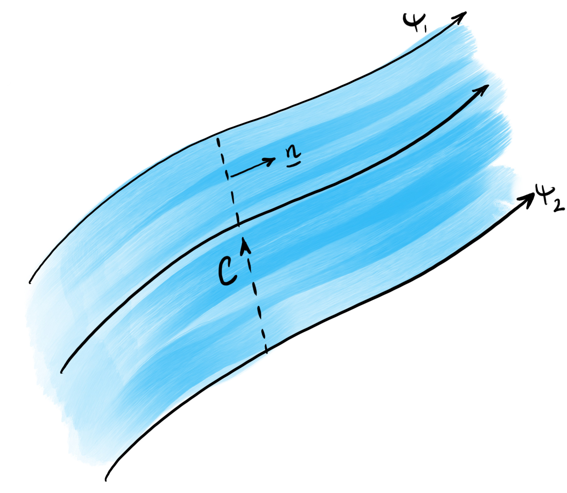
Figure4.2.2.Flow between two streamlines, where the streamlines \(\psi_1\) and \(\psi_2\) are constant. Later, we will consider the flux through the contour \(C\) illustrated in the figure along with its unit normal \(\bn\text{.}\)
The streamfunction is thus constant on streamlines. Consider two streamlines. The following theorem relates the flux between the streamlines to the streamline values.
Consider two streamlines \(\psi = \psi_1\) and \(\psi = \psi_2\text{.}\) We assume that the streamlines pass through the points A and B respectively. Consider a contour \(C\) connecting A and B. The flux (net flow of fluid) through \(C\) and hence between the streamlines is
In the third line above, \([\psi]_C\) is the change of \(\psi\) across the contour. Note that there is somewhat an arbitrary choice of direction for the contour \(C\text{,}\) as related to the selection of the normal direction \(\bn\text{,}\) and the positivity or negativity of the flux. To be safe, we have taken the absolute value in the problem.
where \(a\) is a positive constant. By finding the streamfunction, \(\psi\text{,}\) calculate the volume flux across a curve connecting points \(A = (0, 0)\) and \(B = (1, 1)\) using Theorem 4.2.3.
Finally, note that the velocity potential was governed by Laplace’s equation, \(\nabla^2 \phi = 0\text{.}\) The streamfunction is also governed by the same Laplace’s equation.
Like in the situation of certain flows, e.g. the line source in Example 4.1.7, it is easier to work in alternative coordinate systems to study the streamfunction. Since we know that \(\bu = \nabla \times (\psi \bk)\) by (4.2.3), we can use the conversion of the curl to polar coordinates in (A.1.31) to give
For the situation of the line source in Example 4.1.7, we want to work with polar coordinates. From the previous work, we have for this situation the potential \(\phi = Q/(2\pi log r\text{.}\) It then follows from the polar version of the gradient in (A.1.30), that the velocity is entirely radial and
Then indeed note that the lines of constant \(\psi\) are given by the radial lines of constant \(\theta\text{,}\) matching the illustration in Figure 4.1.8.
Another remark concerns the fact that \(\psi\) is a multi-valued function in the example of the line source Example 4.2.8, gaining a jump of \(Q\) every time the origin is encircled. This is indeed a warning that the standard proof, analogous to Theorem 4.1.1, leading to the existence of a unique streamfunction, via (4.2.4) would not apply since the velocity field Example 4.2.8 is not defined at the origin. However, despite this, we see that the streamfunction provides well-defined predictions of streamlines on the cut plane with e.g. \(\theta \in [0, 2\pi)\text{.}\)
Like the case of the potential function in Example 4.1.9, the linearity of the equation governing the streamfunction implies that we can consider the combination of those streamfunctions for a line source with a uniform flow. This yields
\begin{equation*}
\psi = Uy + \frac{Q}{2\pi}\theta,
\end{equation*}
for the case of uniform flow of speed \(U\) in the positive \(x\)-direction. The streamlines are then given by
\begin{equation*}
Uy + \frac{Q}{2\pi} \theta = \frac{Q}{2\pi}C,
\end{equation*}
having designed the constant combination on the right hand-side for convenience. Then using \(y = r\sin\theta\text{,}\) we have
\begin{equation*}
r = \left(\frac{Q}{2\pi U}\right) \frac{C - \theta}{\sin\theta}.
\end{equation*}
Our previous examples were reliant on considering the flows generated by the velocity potentials studied previously. However, we can also consider "fundamental solutions" of the equation \(\nabla^2 \psi = 0\) in their own right. Recall that in deriving the velocity potential of the line source in Example 4.1.7, we considered the solution of an axi-symmetric problem, where \(\phi = \phi(r)\) is only dependent on the distance from the origin. A similar argument must imply that the analogous axi-symmetric streamfunction is a permissible solution. And this leads us to the following example.
The quantity \(\Gamma\) is called the vortex strength, analogous to the source strength \(Q\) in Example 4.1.7. Let us consider the amount of circulation around a contour \(C\) that contains the origin:
\begin{equation*}
\oint_C \bu \cdot \de{\bx} = \oint_C (u \, \de{x} + v \, \de{y}),
\end{equation*}
i.e. one envisions encircling the origin along \(C\text{,}\) adding up each of the velocity components tangential to the path. This is the circulation. By Stokes’ theorem it is equal to the flux of vorticity of the corresponding bounding surface.
So indeed this gives us an intuitive understanding of \(\Gamma\text{.}\) Notice that \(\Gamma \gt 0\) corresponds to flow in the anticlockwise sense, and \(\Gamma \lt 0\) corresponds to flow in the clockwise sense.