Further, we know that if the flow is irrotational, then there exists a velocity potential, \(\phi\text{,}\) such that \(\bu = \nabla \phi\text{.}\) Thus the velocities are expressed as
\begin{equation}
u = \pd{\phi}{x} \quad \textrm{and} \quad v = \pd{\phi}{y}.\tag{4.1.3}
\end{equation}
The above result about irrotational flows is a standard result in Vector Calculus, but we will re-state the result here for reference, and provide a review of its proof.
Consider a three-dimensional time-dependent velocity field, \(\bu = \bu(\bx, t)\) defined on a simply connected domain \(\bx\in D \subset \mathbb{R}^3 \times \mathbb{R}^+.\)
Then \(\bu\) is irrotational, i.e. \(\nabla \times \bu = 0\) if and only if there exists a scalar potential, defined on \(D \times \mathbb{R}^+\text{,}\) such that \(\bu = \nabla \phi\text{.}\)
where \(C\) is any contour connecting an arbitrary origin point to the point \(\bx\) (changing the origin point will change the "constant" of integration \(\phi_0(t)\)).
We can verify, using the definition of differentiation, and the fundamental theorme of calculus, applied along each of the three coordinate directions, that \(\nabla \phi = \bu\) as desired.
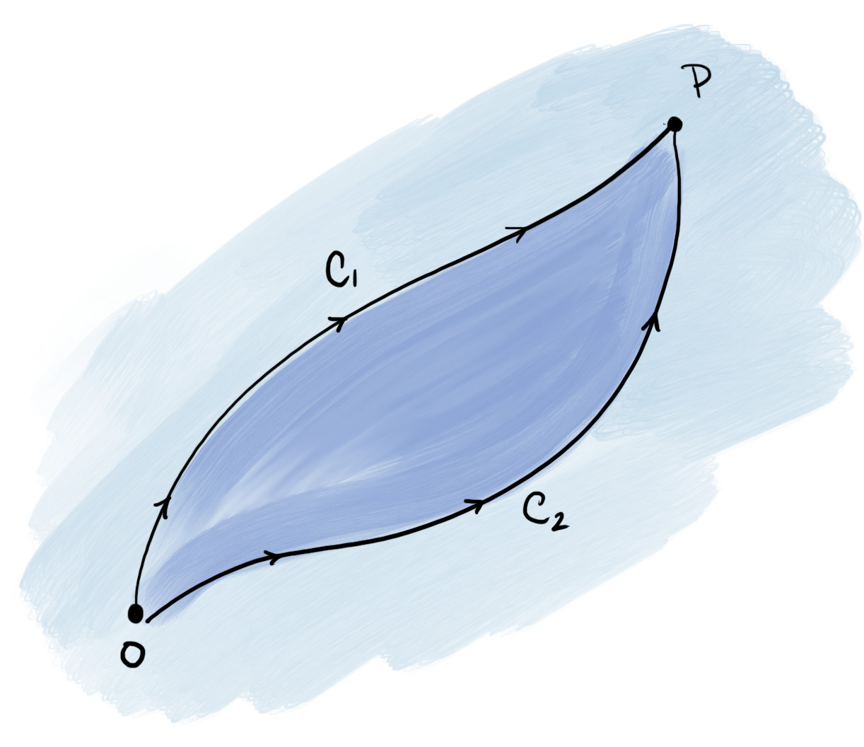
The key is to prove that the above definition is unique, regardless of the choice of contour \(C\text{.}\) To this end, consider two contours, \(C_1\) and \(C_2\text{,}\) both with the same origin point, \(O\text{,}\) and end point \(P\text{.}\) Then the contour \(C_1 - C_2\) is a close contour beginning and ending at \(O\text{.}\)
where \(S\) is any surface with bounding curve \(C_1 - C_2\text{,}\) and with unit normal \(\bn\) positively oriented with the bounding curve. However, the right hand-side is zero by irrotationality, and therefore
within the flow region. This is effectively a single linear equation for the single unknown \(\phi\text{.}\) However, for different problems, the boundary conditions can render even this "simple" problem difficult.
Once the velocity potential \(\phi\) has been solved, the velocities in the flow can be recovered from the relationship (4.1.3). The pressure in the flow also follows from Bernoulli’s equation. For the situation of a steady potential flow, following Theorem 3.5.9, it is
The next three examples will introduce you to the elementary flows consisting of uniform flow, stagnation point flow, and line source/sink flows. You will also investigate the notion of a source "strength".
We aim to derive the potential and velocity for a line source, imagined as the flow consisting of a point source or point sink that ejects/drains fluid from a point in space. Since it would be expected for the potential to be axisymmetric, we attempt to solve \(\nabla^2 \phi = 0\) in plane polar coordinates. This is given by
where we have set an additional constant of integration to zero without loss of generality. The leading constant has been set to \(Q/(2\pi)\) so that \(Q\) can be later identified with a physical quantity.
where the unit vectors written in the Cartesian basis are \(\be_r = [\cos\theta, \sin\theta]\) and \(\be_{\theta} = [-\sin\theta, \cos\theta]\text{.}\) Thus we can write the velocity as
The above corresponds to a velocity field directed radially outwards from the origin. The flow is a called a line source because fluid is ejected from the origin (a source). It refers to a "line" because in \((x, y, z)\text{,}\) the source runs parallel to the \(z\)-axis.
For simplicity, let us take the contour \(C\) to be a circle of constant radius \(r = a\text{.}\) Then since the unit normal is precisely \(\be_r\text{,}\) we have that
Crucially, because the governing fluid mechanical equation is only Laplace’s equation: this is a linear partial differential equation, and therefore the summation of elementary flows also produces an admissible flow.