A reminder of complex variables

Section 1.2 A reminder of complex variables

In Chapter 4, we will leverage the power of complex variables to study certain problems in fluids (flow of a potential flow). One concept that you may be unfamiliar with at this stage is the concept of a branch cut.

🔗

Cover — Figure 1.2.1. An image from Tristan Needham’s "Visual Complex Analysis" [5] showing how complex mappings transform shapes from one region to another.
🔗

Subsection 1.2.1 Basic complex representations

Generally, we write the Cartesian and polar form of a complex number as,

\begin{equation*} z = x + \im y = r\e^{\im\theta}, \end{equation*}

for magnitude \(r > 0\) and angle \(\theta\text{.}\) Below, we will consistently refer to \(z\in\mathbb{C}\text{.}\) The decomposition of the complex exponential is given by Euler’s identity:

\begin{equation} \e^{\im\theta} = \cos \theta + \im \sin\theta.\tag{1.2.1} \end{equation}

🔗

The usual trigonometric functions can be extended to the complex plane by considering their definition in terms of complex exponentials and Euler’s identity. For example, we have

\begin{equation} \cos z = \frac{\e^{\im z} + \e^{-\im z}}{2} \quad \text{and} \quad \sin z = \frac{\e^{\im z} - \e^{-\im z}}{2\im}.\tag{1.2.2} \end{equation}

🔗

Another important function we shall consider is the complex logarithm, defined as

\begin{equation} \log z \equiv \log r + \im \theta,\tag{1.2.3} \end{equation}

where \(z = r\e^{\im\theta}\text{.}\) That this definition is sensible is verified by checking that the logarithm is the inverse of the exponential. That is,

\begin{equation*} \e^{\log z} = \e^{\log r + \im\theta} = \e^{\log r} \e^{\im\theta} = z. \end{equation*}

🔗

However, the definition (1.2.3) is troubling because it is not single-valued. For example, writing \(z = 1 \e^{\im \cdot 0}\) and \(z = 1 \e^{\im \cdot 2\pi}\) gives two different possible values of \(\log z\) for the same value of \(z = 1\text{.}\) We dig deeper into this issue.

🔗

Subsection 1.2.2 Complex functions

A complex function maps points on the complex plane to points on the complex plane. For instance, the square function,

\begin{equation*} f(z) = z^2 = r^2 \e^{2\im \theta}, \end{equation*}

can be better understood by its effect on points on the unit circle, \(|z| = 1\text{.}\)

🔗

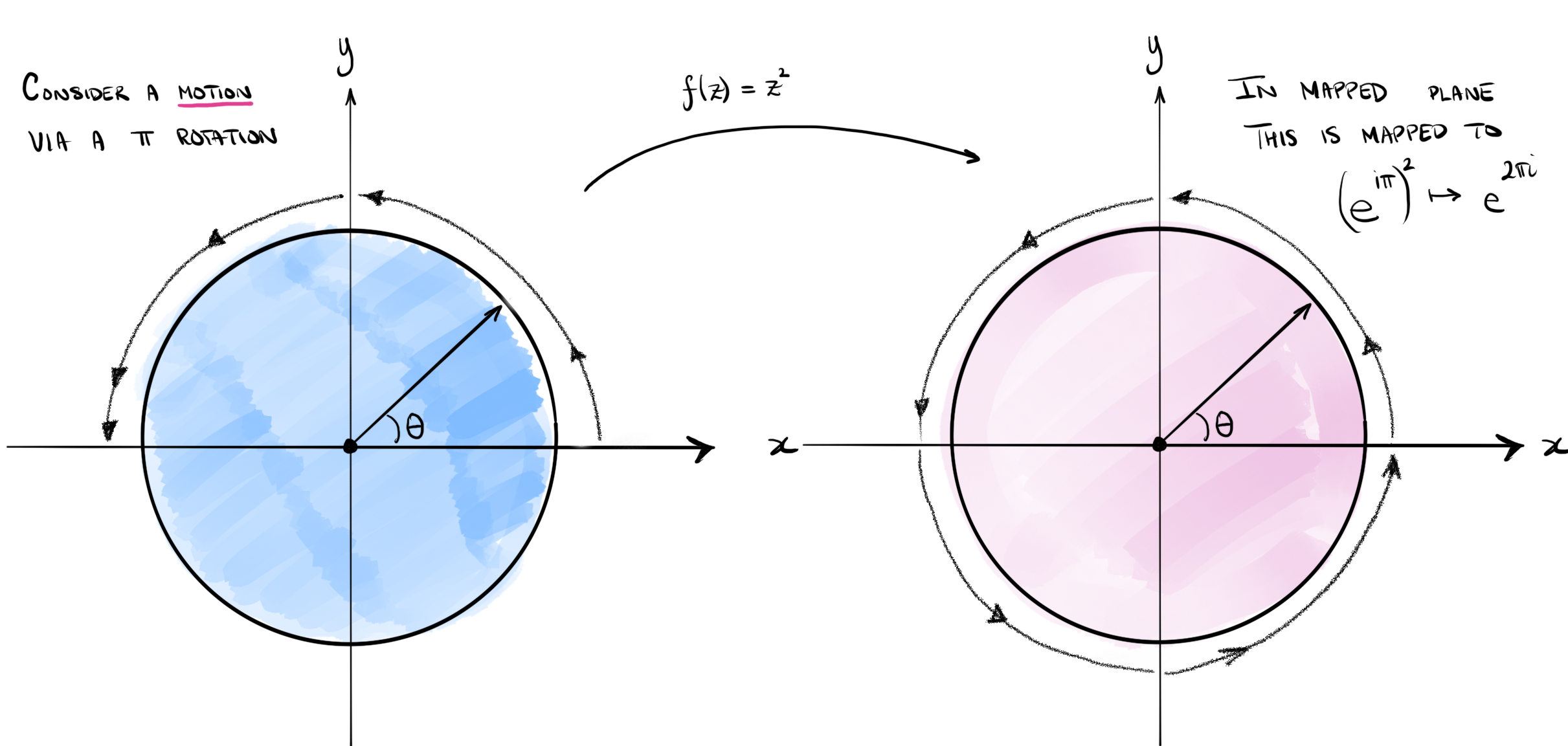
Consider a particle that orbits around the unit circle in the \(z-\)plane at unit speed. If the particle rotates by half a revolution, with \(\theta = \pi\text{,}\) then in the image plane, the image particle has rotated by a full revolution, with \(f(z) = (\e^{\im \pi})^2\) in this same unit time. This is illustrated by the image in Figure 1.2.2.

🔗

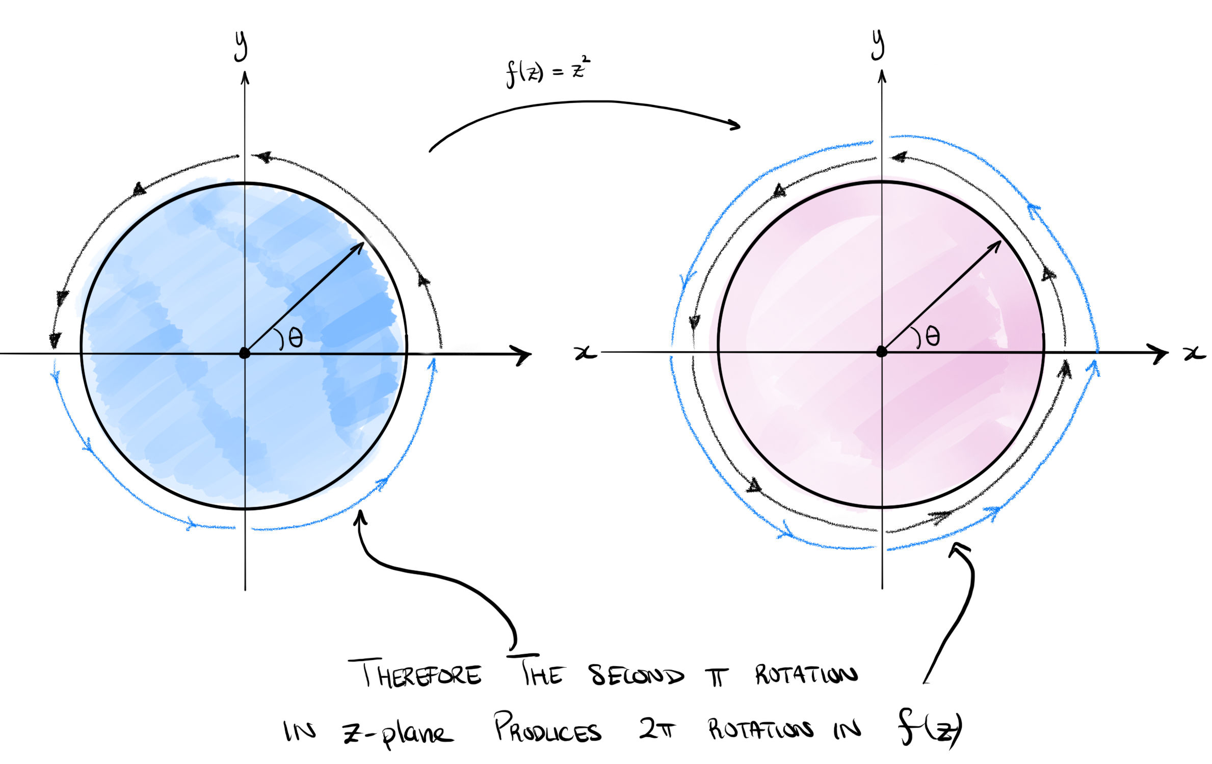
z2 map — Figure 1.2.2. A revolution of \(\pi\) in the pre-image produces a full rotation in the image plane.
🔗

Now we continue rotating around the unit circle in the \(z-\)plane, performing an additional \(\pi\) rotation. Within the image plane, the particle has now completed another full rotation around the unit circle. This is shown in Figure 1.2.3.

🔗

Subsection 1.2.3 Multifunctions, branch cuts, and Riemann sheets

Now consider the inverse function of the above, given by the square root function,

\begin{equation*} f(z) = z^{1/2}. \end{equation*}

🔗

Visually, we can simply consider the same figures as before, but now with the mapping proceeding from the right subfigure to the left subfigure. Observe that there is now an ambiguity, because for each point in the original \(z-\)plane, there are two possible images to assign for \(z^{1/2}\text{,}\) corresponding to either the top semicircle of the left figure, or the bottom semicircle.

🔗

That is, it is unclear of whether we should define:

\begin{equation*} f(z) = z^{1/2} = r^{1/2} \e^{\im\theta/2}, \end{equation*}

\begin{equation*} f(z) = z^{1/2} = -r^{1/2} \e^{\im\theta/2}. \end{equation*}

🔗

Moreover there is a problem, for if we allow a "motion" of the \(z\) values such that \(z\) rotates more than a complete revolution around the origin, then \(f(z)\) is no longer well-defined and takes on multiple possible values.

🔗

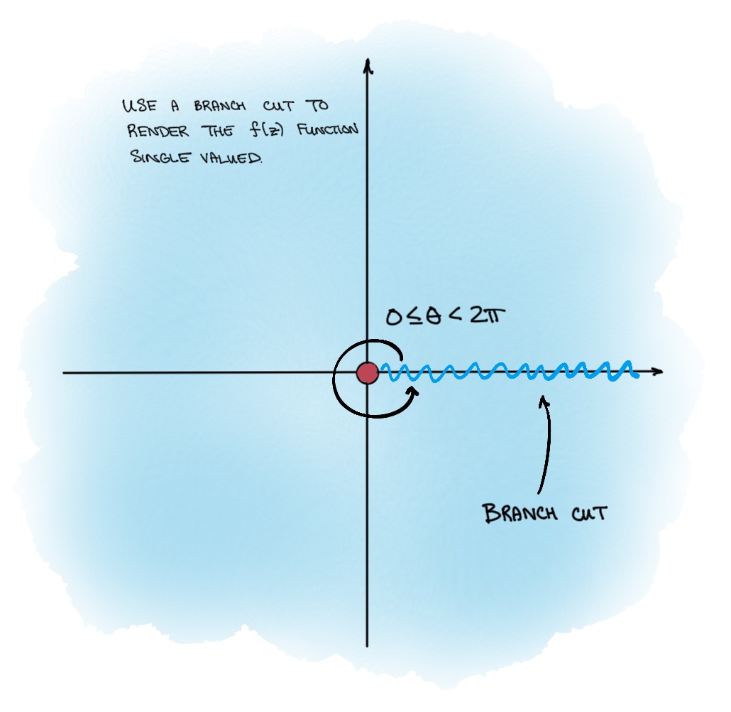
This leads to the following restriction. We define a branch cut of the \(z-\)plane, and restrict the possible argument values. For example, we may choose

\begin{equation*} 0 \leq \theta < 2\pi, \end{equation*}

hence imposing that the branch cut is along the positive real axis. This is illustrated in Figure 1.2.4 where the branch cut is shown as a wavy line.

🔗

Alternatively, we could have equally chosen

\begin{equation*} -\pi \leq \theta < \pi, \end{equation*}

hence taken the branch cut along the negative real axis.

🔗

Once the branch cut has been selected, the previous multi-function is restricted to one of the two possible definitions above. This leads to the definition as follows.

🔗

Definition 1.2.5. Branches of the square root function.

The positive branch of the square root, with branch cut taken along the positive real axis, is defined by

\begin{equation*} f(z) = f_1(z) = z^{1/2} = r^{1/2} \e^{\im\theta/2}, \end{equation*}

for \(r > 0 \) and \(0 \leq \theta < 2\pi\text{.}\) Other branch cut choices can be taken in an analogous manner (curve that extends from \(z= 0\) to \(z = \infty\)).

🔗

Then the above \(f\) with \(z\) restricted as given is a well-defined single-valued function.

🔗

There is an analogous negative branch defined as

\begin{equation*} f(z) = f_2(z) = z^{1/2} = -r^{1/2} \e^{\im\theta/2}, \end{equation*}

🔗

Therefore, \(f_1\) and \(f_2\) make up the two "layers" of the square root function.

🔗

We often refer to each individual "layer" as a Riemann sheet. The critical point \(z = 0\) is referred to as a branch point.

🔗

The collection of Riemann sheets is referred to as a Riemann surface.

🔗

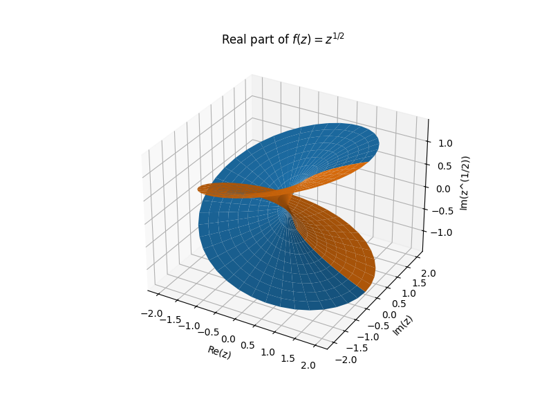
In Exercise 1.3.1, you will plot the Riemann surface that corresponds to \(f(z) = z^{1/2}\text{.}\) The result might look like this version created using Python graphing tool:

Sqrt — Figure 1.2.6. Riemann surface for the square root function. This shows the real part of the square root, which consists of both a positive branch and a negative branch. In the above case, we have placed the branch cut along the negative real axis.
🔗

🔗

A similar argument would indicate that the function

\begin{equation} f(z) = (z + 1)^{1/2} (z - 1)^{1/2},\tag{1.2.4} \end{equation}

requires two branch cuts in general, each cut originating from the two branch points at \(z = \pm 1.\) You will study this function in more detail in Exercise 1.3.2.

🔗

Also in Exercise 1.3.3, you will study the branch structure of the complex logarithm in (1.2.3).

🔗

Subsection 1.2.4 Other functions and visualisations

The theory of complex analysis is rich in different kinds of visualisations. Another way to visualise a complex function is by considering its effect on a gridded pattern in the original \(z\)-plane, and then to imagine the function as warping this pattern. With this interpretation, it will be seen clearly that the operation of \(f(z) = z^2\) essentially rotates and expands the \((x, y)\) plane. This is seen in the following video.

🔗

However, you will also encounter some of these more complex mappings, notably the inversion map, \(f(z) = 1/z\) in Chapter 4.

🔗

The theory in the video (visualisation on the Riemann sphere) is not necessary for this course; it is presented here just out of interest (and because the video is beautiful!).

🔗

Remark 1.2.7.

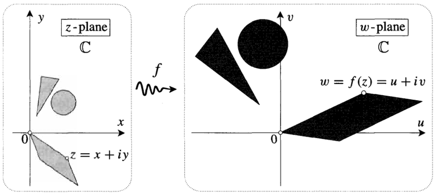
It is sensible to ask: what does this have to do with fluid mechanics?. In Chapter 4, we will see that the use of complex functions can map a region of fluid to another.

🔗

Subsection 1.2.5 Differentiation of complex functions

In this chapter, we will only cover the basic necessities of visualising and studying complex functions. In Chapter 4, we will need additional theory on the differentiation of complex functions.

🔗

Subsection 1.2.6 Summary

Certain complex functions are only well-defined with appropriate branch cuts chosen. However, once such restrictions are made (and an individual Riemann sheet chosen), the complex function is well defined. The branch cut will correspond to locations where the function is nonsmooth (in its real and/or imaginary components).

🔗

Prev Top Next