Viscosity quantifies the fluid’s internal resistance to flow when a force is applied (the higher the resistance the higher the viscosity). One of the most common mathematical models of an idealised fluid is a Newtonian fluid, which will be defined precisely in Section 7.4. For these fluids, the shear viscosity \(\mu\) (sometimes called dynamic viscosity, or just viscosity) is a scalar quantity. In S.I. units, it is measured in \(\textrm{Pa\,s} = \mathrm{kg\,m^{-1}\,s^{-1}}\text{.}\)
Example7.1.1.Thought experiment to measure viscosity.
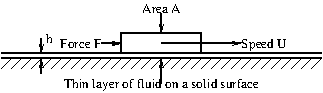
We could imagine a thought experiment to measure the shear viscosity of a fluid as follows, see also Figure 7.1.2. A solid block of area \(A\) floats on the surface of a thin layer of the fluid of thickness \(h\text{.}\) The block is pushed with a force \(F\) parallel to the surface of the fluid, causing it to move with a steady velocity \(U\text{.}\) The shear viscosity is given by
In principle this formula could be used to determine the viscosity of a fluid experimentally; however, in practice it is more common to use a falling ball viscometer (see Exercise 7.9.3 in the worksheet at the end of this chapter).
It is sometimes mathematically more convenient to work in terms of the kinematic viscosity \(\nu\) (measured in \(\mathrm{m^2\,s^{-1}}\)). This is related to the shear viscosity via
The shear viscosity of air increases with increasing temperature, whereas that of water decreases with increasing temperature. This is typical behaviour for gases and liquids, respectively. Many real fluids have more complicated viscosity properties, for example blood, mucus, shampoo, egg white and custard. In this course we mainly consider Newtonian fluids, thereby avoiding a lot of complexity!
Note that we have not yet formally defined the shear viscosity, although the example given in Example 7.1.1 provides an informal definition. This concept will be formalised in Section 7.3.
This is one of the most important flow parameters in the study of fluid dynamics, as its order of magnitude determines many of the qualitative features of the flow. In a given flow, it quantifies the relative importance of inertial and viscous effects.
The Reynolds number is a dimensionless quantity, defined by
\begin{equation*}
\textrm{Re} = \frac{\rho U L}{\mu} = \frac{U L}{\nu},
\end{equation*}
where \(U\) is a characteristic (or typical) velocity of the flow and \(L\) is a characteristic lengthscale. It equals the typical size of an inertial acceleration divided by a typical size of a viscous acceleration in the flow.
What do we pick as the characteristic length and velocity scales? This is something that gets easier with increasing experience. For a given problem there are usually ‘natural’ scales that arise within it.
As an illustrative example of how we might think about choosing suitable scales, consider a steady flow along a pipe with a circular cross-section. An appropriate choice of \(L\) could be the pipe radius or diameter, while an appropriate value of \(U\) could be the velocity along the centreline (axis) of the pipe or the average velocity across the pipe cross-section (equal to the volumetric flux (volume per unit time) of fluid passing along the pipe divided by the cross-sectional area of the pipe).
Different choices of scales (for example radius vs. diameter and centreline vs. average velocity in the pipe example given in Remark 7.1.7) would lead to different numerical values of \(\textrm{Re}\text{.}\) However, note:
The order of magnitude of the Reynolds number is the same for all choices. Thus, when describing a flow, the value of \(\textrm{Re}\) is often quoted as an order-of-magnitude property.
If we give detailed information about exactly which length and velocity scales are being used then we can directly compare different values of \(\textrm{Re}\text{,}\) even if they are of the same order of magnitude. For example, we might do this in a plot of a property of the flow against the Reynolds number. In this case, it would be good scientific practice to specify the choice of velocity and length scales used.
Remark7.1.8.Flow characteristics at different Reynolds numbers.
Typical characteristics of the flow are strongly associated with the order of magnitude of the Reynolds number:
Low-Reynolds-number flows (\(Re \ll 1\)):
Examples include several biological examples, such as flow in capillaries (the smallest blood vessels) swimming bacteria or other single cell organisms, lymphatic system flow, and other examples include microfluidics, glacier flow, and spreading honey on toast.
Low-Reynolds-number flows are also reversible, meaning that if a force is applied, followed by the reverse of that force then the fluid particles return to their original positions. This movie shows a low-Reynolds-number flow that is reversible, whereas this movie shows a flow with a higher Reynolds number that is not reversible.
Flows with moderate Reynolds number (\(1 \ll Re \ll 2{,}000\)):
Examples include flows in most blood vessels that are not capillaries, small fish swimming, not-too-fast flow out of a domestic tap, stirring a cup of tea.
Flows in pipes with moderate Reynolds number are often described as laminar, meaning that the fluid moves in ‘layers’ sliding past each other (in fluid dynamics, the word ‘laminar’ is often used to mean that the flow is not turbulent).
High-Reynolds-number flows (typically \(Re\) above about \(1{,}000\)):
Examples include atmospheric and ocean flows, rivers, large industrial processes, flows around vehicles, airflow in trachea and ships or large animals swimming.
This is a qualitative type of flow that is characterised as having many different length scales, and the flow is mathematically chaotic. Chaotic flow means that fluid particles that start close together can become widely separated over time. As well as the scale of the whole experiment, the turbulence has eddies on all small length scales. Turbulent flows are analysed mathematically by decomposing the fluid velocity into a mean flow, which describes the large-scale flow and a fluctuating flow, which describes the eddies. Equations can be written for each of these, but this decomposition leads to the so-called closure problem, in which an assumption needs to be made to provide a final equation that governs the dynamics.
Turbulence is of great importance in applications such as aeronautical engineering, weather forecasting and large-scale industrial flows, basically because large and fast moving flows have a sufficiently high Reynolds number that turbulence is unavoidable and it dominates the flow characteristics.
In addition to the balances implied by mass and momentum conservation that you have so far been working on in this course, there is an additional condition needed, and this is called a state relation. This relates the thermodynamic variables density \(\rho\text{,}\) pressure \(p\) and temperature \(T\text{.}\) In this section, we give two of the most common state relations that are used mathematically, the first for liquids and the second for gases.
Liquids are often assumed to be incompressible, that is we assume \(\rho = \textrm{constant}\text{.}\) This is the most common assumption made in this course. However, it is important to be aware that it is not always appropriate.
One of the most common reasons that making the assumption \(\rho = \textrm{constant}\) does not capture the flow dynamics accurately is if there are significant temperature variations within the liquid. Typically, liquids expand as the temperature rises, and this leads to thermal convection, which needs to be taken into account in the mathematical analysis.
In a problem in which temperature variations are important in the fluid dynamics, it is often sufficient to assume the Boussinesq approximation:
In the buoyancy term of the momentum conservation equation (that is the term \(\rho g\) appearing in the Euler equation), we assume the density is a linear function of the temperature. Thus we write
In fluid dynamics the form (7.1.1) is more convenient than \(pV=nRT\) because it can be applied at each point in the gas, whereas \(pV=nRT\) is a law applying to a fixed finite volume.