Flow visualisation, fluxes, and forces

Section 2.2 Flow visualisation, fluxes, and forces

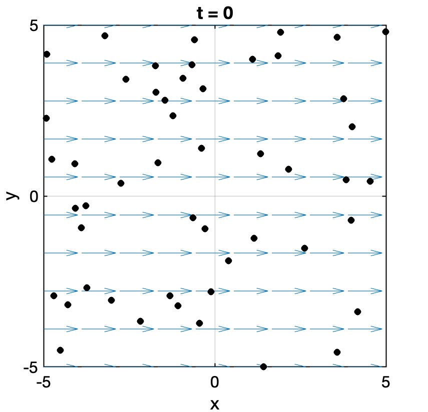
There are different ways to visualise the dynamics of a fluid. Given the velocity, $\bu(\bx, t)\text{,}$ we can plot a vector field at each point in space, and at a fixed moment in time. Little arrows are used to indicate the direction and the length of the arrow can be chosen to represent the magnitude. Joining these up at a fixed moment in time into smooth curves gives the streamlines of the flow. This is often the easiest type of visualisation to perform mathematically, but the hardest experimentally.

🔗

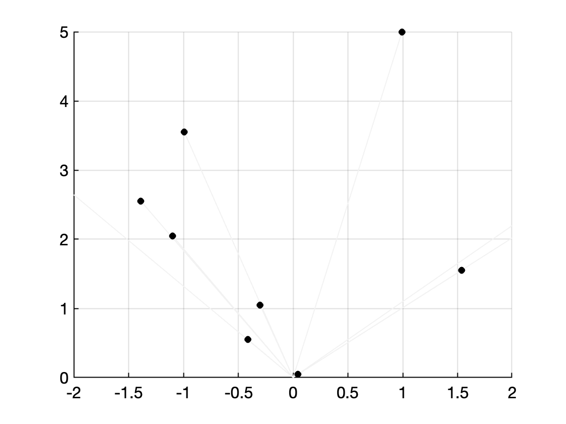
Another representation of the flow is using particle paths or pathlines. Given a point and time, the particle path is the trajectory that would result if a particle were dropped into the flow at that chosen point and time. It is thus found by solving an equation where at every point on the trajectory, the particle’s velocity is the specified velocity of the fluid.

🔗

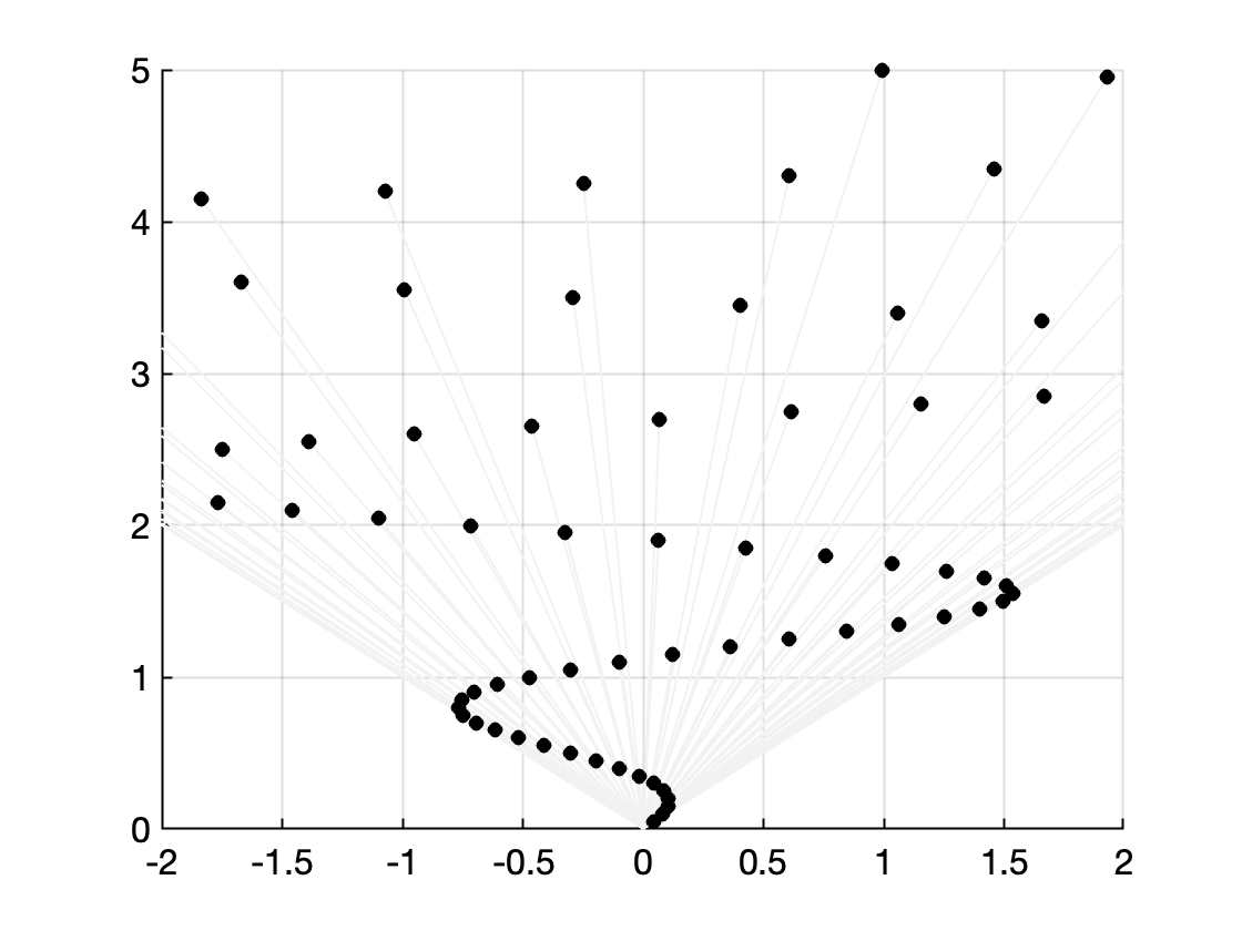
A third representation is a streakline. If dye were continuously released into a fluid from a fixed chosen point, the streakline at a given time is the line that would be made by the dye. It is thus found by finding the current position of those particles whose pathline has visited the chosen point at any past time. This is often the easiest type of visualisation to perform experimentally, but the hardest to perform mathematically.

🔗

Note that in a steady flow, the streamlines, pathlines and streaklines all coincide. However, in an unsteady flow, they are all different. In Exercise 2.3.1 you will study a video showing this concept.

🔗

Subsection 2.2.1 Definitions of streamlines, pathlines, streaklines

In the definition below, we define these concepts more concretely.

🔗

Definition 2.2.1. Particle streamlines.

Consider a fixed time, $t = t_1\text{.}$

🔗

Select an initial point, $\bx_1$ at this time.

🔗

The streamline, $\bx = \bx(s)$ through the above point is given by solving the parametric equation

\begin{equation*} \dd{\bx}{s} = \bu(\bx(s), t_1), \quad \text{with $\bx(s = 0) = \bx_1$,} \end{equation*}

where $s$ is a parameter along the streamline. Choosing a variety of different initial points, $\bx_1\text{,}$ and solving the above equation gives a family of streamlines at time $t_1\text{.}$

🔗

Basically, given a velocity field, we freeze time. The streamlines are those curves that are traced out by the velocity field in the "snapshot".

🔗

Definition 2.2.2. Pathline or particle path.

Consider now a particle that begins at the location $\bx_2$ at time $t = 0\text{.}$

🔗

We consider the partical path or pathline of the particle, given by the curve $\bx = \bx(t)$ and found by solving the equation

\begin{equation*} \dd{\bx}{t} = \bu(\bx(t), t), \quad \text{with $\bx(0) = \bx_2$.} \end{equation*}

Choosing a variety of initial points, $\bx_2\text{,}$ yields a family of pathlines.

🔗

The pathline or particle path from an initial point is what we would physically expect if we were to dye the point with a colour and follow the dye colour as time increases.

🔗

Definition 2.2.3. Streakline.

Consider now fixing a location $\bx_3\text{.}$

🔗

The streakline for a point $\bx_3$ is given by solving the equation

\begin{equation*} \dd{\bx}{t} = \bu(\bx(t), t), \qquad \textrm{with $\bx(t_3) = \bx_3$}, \end{equation*}

for a variety of values of $t_3\text{.}$ This gives the current position of all particles that have passed through the point $\bx_3$ at any time $t_3$ in the past.

🔗

If it is the case that the velocity is time independent, i.e. $\bu = \bu(\bx)\text{,}$ then the three above definitions coincide.

🔗

You will practice the theory of these concepts in Exercise 2.3.5 and do a worked example in Exercise 2.3.6 of the problem set.

🔗

Subsection 2.2.2 Examples of streamlines, pathlines, and streaklines

Let us practice these concepts.

🔗

Example 2.2.4. Stagnation point flow.

Consider a fluid described by the two-dimensional velocity field

\begin{equation*} \bu(\bx, t) = (x, -y, 0). \end{equation*}

Derive and plot the streamlines of the flow. Discuss what occurs with particle paths and streaklines.

🔗

Solution.

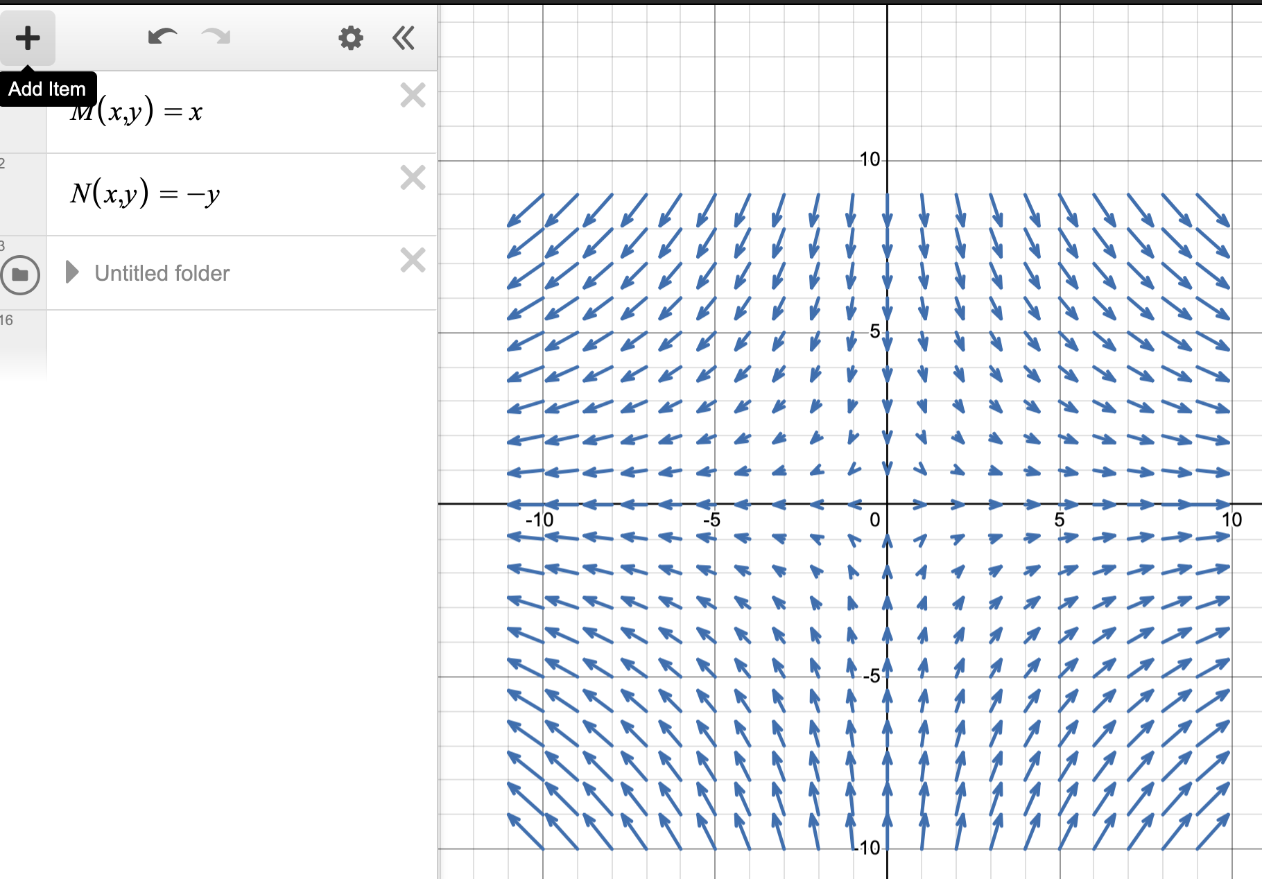
There are many online applications, such as this one that will allow you plot a two-dimensional direction field. It is also good to do it yourself by hand.

🔗

The streamlines follow from Definition 2.2.1. We seek to solve the equations

\begin{align*} \dd{x}{s} &= x, \\ \dd{y}{s} &= -y, \\ \dd{z}{s} &= 0. \end{align*}

Solving thus gives $x = A \e^s, y = B\e^{-s}, z = C,$ for constants $A, B, C\text{.}$

🔗

You can put initial conditions to determine the constant and plot the trajectories for different values of $s\text{.}$

🔗

However, in this case, it is easier to remove the time-like variable, $s\text{,}$ entirely. Notice that

\begin{equation*} xy = AB = \textrm{constant}. \end{equation*}

Therefore, the trajectories lie along hyperbolae.

🔗

Notice that in this case, the velocity field is time-independent, and therefore the particle paths coincide with the streamlines and streaklines.

🔗

For instance, the particle path through a particle at $\bx_2 = (1, 1, 0)$ is given by (replacing $s$ with $t$):

\begin{equation*} \bx(t) = (\e^t, \, \e^{-t}, \, 0). \end{equation*}

Similarly, the streakline through the point $(1, 1, 0)$ is precisely the set of points above.

🔗

Example 2.2.6. Straight streamlines and circular pathlines.

Consider the unsteady flow given by

\begin{equation*} \bu(\bx, t) = (\cos t, \sin t, 0)\text{.} \end{equation*}

Plot the streamlines of the flow on the plane $z = 0\text{,}$ and also the particle trajectories. What occurs with the streaklines?

🔗

Answer.

In this case, the velocity field is changing in time. Consider firstly the concept of the streamline in Definition 2.2.1.

🔗

We solve the governing equations for the streamlines $\bx = \bx(s)\text{,}$

\begin{equation*} \dd{x}{s} = \cos t, \quad \dd{y}{s} = \sin t, \quad \dd{z}{s} = 0, \end{equation*}

for fixed $t\text{.}$

🔗

This gives

\begin{equation*} x(s) = A + s \cos t, \quad y(s) = B + \sin t, \quad z(s) = C, \end{equation*}

for constants $A, B, C\text{.}$ Therefore the streamline are given by straight lines in the $(x, y)$ plane, if $z = C$ is fixed.

🔗

Consider instead the definition of particle paths via Definition 2.2.2. We seek to solve

\begin{equation*} \dd{x}{t} = \cos t, \quad \dd{y}{t} = \sin t, \quad \dd{z}{t} = 0, \end{equation*}

yielding

\begin{equation*} x(t) = A + \sin t, \quad y(t) = B - \cos t, \quad z(t) = C, \end{equation*}

for constants $A, B, C\text{.}$ Therefore, we see that the particle paths are closed circles (in the $xy$-plane) of unit radius encircling the point $(A, B, 0)\text{.}$

🔗

The fact that the streamlines are straight lines while the particle paths are circular can be visualised in Figure 2.2.7

🔗

Animation of streamlines — Figure 2.2.7. Streamlines and particle paths
🔗

In this case, considering the streakline via Definition 2.2.3, we conclude that the streakline coincides with the particle path. Can you reason why this must be the case in this situation? What is necessary in order for this not to be true?

🔗

Example 2.2.8. An oscillating hose/plate.

Water flows out of an oscillating sprinkler head, held along the edge $y = 0\text{,}$ such that the velocity field produced is given by

\begin{equation*} \bu = [u_0 \sin[\omega(t - y/{v_0})], v_0], \end{equation*}

where $u_0$ and $v_0$ are constants.

🔗

Determine the streamline that passes through the origin at $t = 0$ and $t = \pi/(2\omega)\text{.}$

🔗

Determine the pathline of the particle that was at the origin at $t = 0\text{;}$ at $t = \pi/2\text{.}$

🔗

Qualitatively describe the shape of the streakline that passes through the origin?

🔗

Answer.

gif — Figure 2.2.9. Isolated pathlines show that particles move along straight paths.
🔗

gif — Figure 2.2.10. However, viewed in terms of the streakline, the visible pattern is oscillatory.
🔗

🔗

Subsection 2.2.3 Fluxes and forces

Before we go on, we remind the reader of two important quantities that will be used in the following chapters. These are typicaly introduced in the prior modules on vector calculus.

🔗

The first is the notion of flux through a surface. Given a surface $S$ and a velocity field $\bu\text{,}$ the flux through the surface is the amount of flow through the surface per unit time. It is given by the integral

\begin{equation} \text{flux through $S$} = \iint_S \bu \cdot \bn \, \de{S},\tag{2.2.1} \end{equation}

and $\bn$ is the outer unit normal.

🔗

In 2D, the flux due to a 2D velocity field can also be written as

\begin{equation} \text{flux through $C$} = \int_C \bu \cdot \bn \, \de{s}.\tag{2.2.2} \end{equation}

In the two above formulae, refer to your previous vector calculus notes for the procedures to calculate the area element $\de{S}$ or the line element $\de{s}\text{.}$

🔗

Finally, we may like to also calculate the total force on a surface or on a contour. If $\bF$ is the pointwise force applied at every point, the total force is given by

\begin{equation} \textrm{Total force} = \iint_S \bF \, \de{S}.\tag{2.2.3} \end{equation}

The above remains a vector quantity.

🔗

Prev Top Next