Logo image

Exercises 2.3 Exercises

The kinematics chapter covered the basic essentials about the measurement and computation of fluid velocities and acceleration. We examined the difference between Eulerian and Lagrangian coordinates and derivatives. Examples of streamlines and velocity fields were examined.

1. Flow visualisation.

(a)

Name a few ways in which a fluid flow can be visualised (i.e. how does one produce, in an experiment, such a visualisation?)

(b)

Define, in words, what pathline, streakline, timeline, and streamline means. At 6:30, the author comments that "there is no way to make a streamline visible". Discuss this point.

(c)

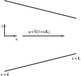
Give the example, shown in the video, where the pathline, streakline, and streamlines all coincide. Draw pictures to illustrate the concept.

(d)

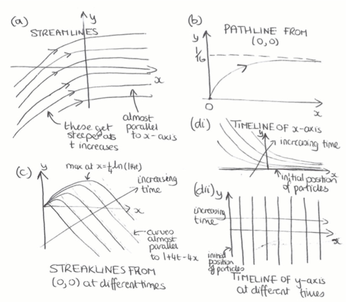
Give an example, shown in the video, where the pathline, streakline, and streamlines do not coincide. Draw pictures to illustrate the concept.

(e)

In the video, an intuitive explanation is given for what it means for the velocity to be incompressible. What is this explanation? (near 8:25)

2. Derivation of the material derivative.

Prove the Eulerian representation of the material derivative, as presented in Theorem 2.1.6 by manually expanding the components of the function. That is, consider a scalar function \(f(\bx, t)\text{.}\) Let the spatial coordinate follow \(\bx = \bx(\bX,t)\) and hence is defined by a specified material label \(\bX\text{.}\) Then derive the identity for
\begin{equation*} \DD{f}{t} = \pd{f}{t} \biggr\rvert_{\bX}, \end{equation*}
according to Definition 2.1.4.
Solution.
This is the chain rule. Denote the three components of \(\bx = (x_1, x_2, x_3)\text{.}\) Then we differentiate through both outer arguments of \(f\text{:}\)
\begin{align*} \pd{f(\bx(\bX, t), t)}{t}\biggr\rvert_{\bX} &= \pd{f}{t}\biggr\rvert_{\bx} + \sum_{i=1}^3 \pd{x_i(\bX, t)}{t}\biggr\rvert_{\bX} \pd{f}{x_i} \end{align*}
The factor,
\begin{equation*} \pd{x_i}{t}\biggr\rvert_{\bX} = \dd{x_i}{t} \equiv u_i, \end{equation*}
corresponds to the velocity component in each direction. Then
\begin{equation*} \pd{f(\bx(\bX, t), t)}{t}\biggr\rvert_{\bX} = \pd{f}{t} + \bu \cdot \nabla f, \end{equation*}
as desired.

3. Eulerian and Lagrangian descriptions.

A velocity field is described in Eulerian terms in Cartesian coordinates by \(\mathbf{u}=(-y,x)\text{.}\)

(a)

What is the Lagrangian position of the particle that starts at the point \((x_0,y_0)\text{?}\) Describe its path. What is its velocity?
Solution.
A particle moves with the velocity of the fluid. Then it must satisfy the equations
\begin{equation*} \dd{x}{t} = -y(t),\quad \dd{y}{t} = x(t) \quad\Rightarrow\quad \dd{^2x}{t^2} = -\dd{y}{t} = -x(t). \end{equation*}
Trying solutions of the form \(x(t)=\e^{\lambda t}\) gives \(\lambda=\pm i\text{,}\) so the general solution is
\begin{equation*} x(t) = Ae^{it}+Be^{-it}, \end{equation*}
or, equivalently,
\begin{equation*} x(t) = C\cos t + D\sin t, \end{equation*}
where \(C\) and \(D\) are constants, and
\begin{equation*} y(t) =-\dd{x}{t}= C\sin t - D\cos t. \end{equation*}
Setting \(x(0)=x_0\) and \(y(0)=y_0\) gives \(C=x_0\) and \(D=-y_0\text{,}\) so
\begin{equation*} \bx(t) = (x_0\cos t - y_0\sin t, x_0\sin t + y_0\cos t). \end{equation*}
This is a circular path of radius \(\sqrt{x_0^2+y_0^2}\) going anticlockwise around the origin. The velocity is
\begin{equation*} \bu(t) = (-x_0\sin t - y_0\cos t, x_0\cos t - y_0\sin t). \end{equation*}

(b)

Express the position and velocity in polar coordinates. What do you notice?
Hint.
Note that
\begin{equation*} \hat{\boldsymbol{r}}= \left(\begin{matrix} \cos\theta\\\sin\theta \end{matrix}\right) =\cos\theta\boldsymbol{i}+\sin\theta\boldsymbol{j}, \quad \hat{\boldsymbol{\theta}}= \left(\begin{matrix} -\sin\theta\\\cos\theta \end{matrix}\right) =-\sin\theta\boldsymbol{i}+\cos\theta\boldsymbol{j}, \end{equation*}
see also (A.1.5), (A.1.6) and (A.1.7).
Solution.
The calculation works out more simply in polar coordinates; the velocity field is
\begin{equation*} \bu = r\be_\theta, \end{equation*}
where \(\be_{\theta}\) is the angular unit vector given in (A.1.6). Then the equation for particle paths is
\begin{equation*} \dd{r}{t} = 0,\quad\dd{r\theta}{t}= r\quad\Rightarrow\quad \dd{\theta}{t}=1. \end{equation*}
Thus \(r(t)=r_0=\sqrt{x_0^2+y_0^2}\) and \(\theta(t)=\theta_0+t\text{,}\) where \(\theta_0=\tan^{-1}(y_0/x_0)\text{.}\) The velocity is \(\bu(t)=r_0\be_{\theta}(t)\text{.}\)
Note that the expression for the velocity in polar coordinates is simpler than that in Cartesian coordinates, being in one coordinate direction only. Performing this conversion makes it easier to find pathlines and streamlines.
This flow is an example of rigid-body rotation, that is the fluid is moving with a velocity field that would be attainable for a rigid body, and there is no relative motion of the fluid particles.

4. Eulerian and Lagrangian descriptions.

A fluid flows through the nozzle shown from \(x=0\) to \(x=L\) with one-dimensional velocity
\begin{equation*} u=U\left(1+\frac{x}{L}\right) \end{equation*}
in the \(x\)-direction, where \(U\) and \(L\) are constants. Note that, in reality the flow would be two- or three-dimensional, but we ignore this here for simplicity.
Figure 2.3.1. Sketch of nozzle.

(a)

What is the particle acceleration?
Solution.
\begin{align*} \ba=&\DD{\bu}{t} \\ =& \pd{\bu}{t} + (\bu \cdot \nabla) \bu\\ =&0+\left(u\pd{u}{x}+v\pd{u}{y}+w\pd{u}{z}\right)\be_x +\left(u\pd{v}{x}+v\pd{v}{y}+w\pd{v}{z}\right)\be_y +\left(u\pd{w}{x}+v\pd{w}{y}+w\pd{w}{z}\right)\be_z\\ =& u\pd{u}{x}\be_x\\ = & U\left(1+\frac{x}{L}\right)\frac{U}{L}\be_x\\ = & \frac{U^2}{L}\left(1+\frac{x}{L}\right)\be_x \end{align*}

(b)

If a particle starts at \(x=0\) at time \(t=0\text{,}\) what is its position at time \(t\text{?}\)
Solution.
We have
\begin{equation*} \dd{x}{t}=u(x)=U\left(1+\frac{x}{L}\right). \end{equation*}
Solving by separation of variables gives,
\begin{align*} &\int_0^x\frac{dx}{1+x/L}=\int_0^t U\,dt\\ \Rightarrow\quad& L\ln\left(1+\frac{x}{L}\right)=Ut\\ \Rightarrow\quad& x(t)=L\left(\e^{Ut/L}-1\right). \end{align*}

(c)

What is its Lagrangian velocity as a function of time?
Solution.
The velocity is
\begin{align*} \dd{x}{t}=&\dd{}{t}\left(L\left(\e^{Ut/L}-1\right)\right)\\ =& L\frac{U}{L}\e^{Ut/L}\\ =& U\e^{Ut/L}. \end{align*}

(d)

What is its Lagrangian acceleration as a function of time?
Solution.
The acceleration is
\begin{align*} \dd{^2x}{t^2}=&\dd{}{t}\left(U\e^{Ut/L}\right)\\ =& \frac{U^2}{L}\e^{Ut/L}. \end{align*}

(e)

Write the Lagrangian velocity and acceleration as a function of \(x\text{.}\) Compare with the corresponding Eulerian velocity and particle acceleration. What do you notice?
Solution.
The velocity is
\begin{equation*} U\e^{Ut/L}=U\left(1+\frac{x}{L}\right), \end{equation*}
as expected. This is the same as the Eulerian velocity at the particle position. The acceleration is
\begin{align*} \frac{U^2}{L}\e^{Ut/L}=&\frac{U^2}{L}\left(1+\frac{x}{L}\right), \end{align*}
which is the same as the particle acceleration, as expected from the defintion.

(f)

How long does it take for a particle to travel from \(x=0\) to \(x=L\text{?}\)
Solution.
The particle reaches \(x=L\) when
\begin{align*} & L\left(\e^{Ut/L}-1\right)=L\\ \Rightarrow\quad& \e^{Ut/L}=2\\ \Rightarrow\quad& t=\frac{L}{U}\ln(2). \end{align*}

5. Particle paths and streamlines.

(a)

Define the particle paths and streamlines for a velocity field \(\bu(\bx,t)\text{.}\) When do these coincide?
Answer.
Particle paths are the trajectories of individual fluid particles, which are found by solving the ODE
\begin{equation*} \dd{\bx}{t} = \bu(\bx,t). \end{equation*}
Streamlines are curves that are instantaneously tangent to the velocity field, and therefore satisfy
\begin{equation*} \dd{\bx}{s} = \bu(\bx,t), \end{equation*}
where \(s\) is a parameter along the streamline. The two coincide if the flow is steady, i.e. \(\bu(\bx,t)=\bu(\bx)\text{.}\)

(b)

By drawing a sketch of a pathline and considering the points \(\bx\) where the particle is at time \(t\) and \(\bx+\de\bx\) at time \(t+\de t\text{,}\) show that a quantity \(f(\bx,t)\) is preserved following the flow if
\begin{equation*} \DD{f}{t}=\pd{f}{t}+\bu\cdot\nabla f=0. \end{equation*}
Hint.
We can write \(\de\bx=\bu(\bx,t)\de t+\dots\text{,}\) where "\(\dots\)" indicates smaller corrections. We need to find
\begin{equation*} \DD{f}{t}=\lim_{\de t\rightarrow0}\frac{f(\bx+\de\bx,t+\de t)-f(\bx,t)}{\de t}. \end{equation*}
Now write \(f(\bx+\de\bx,t+\de t)\) as a Taylor series about \(f(\bx,t)\) and use this to simplify the above expression.
Answer.
Figure 2.3.2. Pathline, showing the particle positions at times \(t\) and \(t+\de t\text{.}\)
Figure 2.3.2 shows the points \(\bx(t)\) and \(\bx(t+dt)=\bx(t)+\de\bx\text{,}\) and the equation for pathlines gives \(\de\bx=\bu(\bx,t)\de t\text{.}\) We follow the value of \(f\) following a particle:
\begin{align*} \dd{f}{t}&=\lim_{\de t\rightarrow0}\frac1{\de t}\left(f(\bx+\de\bx,t+\de t)-f(\bx,t)\right)\\ &=\lim_{\de t\rightarrow0}\frac1{\de t}\left(f(\bx,t)+\de\bx\cdot\nabla f(\bx,t)+\de t\pd{f}{t}(\bx,t)+\dots-f(\bx,t)\right)\\ &=\lim_{\de t\rightarrow0}\frac1{\de t}\left(\bu(\bx,t)\de t\cdot\nabla f(\bx,t)+\de t\pd{f}{t}(\bx,t)+\dots\right)\\ &=\pd{f}{t}+\bu\cdot\nabla f=\DD{f}{t}, \end{align*}
(’’\(\dots\)’’ denotes higher order terms). Thus the value is preserved if \(\DD{f}{t}=0\text{.}\)

(c)

In a similar way, show that \(f\) is constant along streamlines if
\begin{equation*} \bu\cdot\nabla f=0. \end{equation*}
Hint.
In this case we can consider the points \(\bx\) and \(\bx+\de\bx\) on the streamline, where \(\de\bx=\bu(\bx,t)\de s+\dots\text{,}\) where "\(\dots\)" indicates smaller corrections. We need to find
\begin{equation*} \dd{f}{s}=\lim_{\de s\rightarrow0}\frac{f(\bx+\de\bx,t)-f(\bx,t)}{\de t}. \end{equation*}
Now write \(f(\bx+\de\bx,t)\) as a Taylor series about \(f(\bx,t)\text{.}\)
Answer.
Now suppose that in Figure 2.3.2, we have shown instead the situation of a streamline.
In this case, the points \(\bx(s)\) and \(\bx(s+ds)=\bx(s)+\de\bx\) are shown, and the equation for streamlines gives \(\de\bx=\bu(\bx,t)\de s\text{.}\) We follow the value of \(f\) along the streamline:
\begin{align*} \dd{f}{s}&=\lim_{\de s\rightarrow0}\frac1{\de s}\left(f(\bx+\de\bx,t)-f(\bx,t)\right)\\ &=\lim_{\de s\rightarrow0}\frac1{\de s}\left(f(\bx,t)+\de\bx\cdot\nabla f(\bx,t)-f(\bx,t)\right)\\ &=\lim_{\de s\rightarrow0}\frac1{\de s}\left(\bu(\bx,t)\de s\cdot\nabla f(\bx,t)\right)\\ &=\bu\cdot\nabla f. \end{align*}
Thus the value of \(f\) is preserved if \(\bu\cdot\nabla f=0\text{.}\)

6. Streamlines, pathlines and streaklines.

The velocity of a two-dimensional fluid flow in Cartesian coordinates is \(u = 1\text{,}\) \(v = t e^{-4x}\text{.}\) Calculate and sketch the following:

(a)

the streamlines at a fixed time \(t > 0\text{,}\)
Answer.
The streamlines are given by
\begin{equation*} \pd{y}{x}=te^{-4x}\quad\Rightarrow\quad y=y_0-\frac{t}{4} e^{-4x}, \end{equation*}
for any constant \(y_0\text{.}\) Different values of \(y_0\) give different streamlines. See Figure 2.3.3 for a sketch.
Figure 2.3.3. Sketch of streamlines, pathline and streaklines.

(b)

the pathline of the particle starting from \((x_0,y_0)\text{.}\) Hence find and sketch the pathline of the particle that starts from \((0,0)\text{,}\)
Answer.
The pathlines for a particle starting from \((x_0,y_0)\) are given by
\begin{align*} &\dd{x}{t}=1,\quad \dd{y}{t}=te^{-4x}\\ \Rightarrow\quad& x = x_0 + t,\quad y = y_0 + \frac{1}{16} e^{-4x_0} - \frac{1+4t}{16} e^{-4(x_0+t)}. \end{align*}
Eliminating \(t\text{:}\)
\begin{equation*} y = y_0 + \frac{1}{16} e^{-4x_0} - \frac{1+4x-4x_0}{16} e^{-4x}. \end{equation*}
This is a general pathline. For the particular particle that starts from \((0,0)\text{:}\)
\begin{equation*} y = \tfrac{1}{16}\left(1 - (1+4x)e^{-4x}\right). \end{equation*}
See Figure 2.3.3 for a sketch.

(c)

and the streaklines passing through \((0,0)\text{.}\)
Hint.
The expression for a general pathline starting from \((x_0,y_0)\) is given by
\begin{equation*} x = x_0 + t,\quad y = y_0 + \frac{1}{16} e^{-4x_0} - \frac{1+4t}{16} e^{-4(x_0+t)}. \end{equation*}
Answer.
Suppose the particle that started at \((x_0,y_0)\) hits the special point \((0,0)\) at time \(t_1\text{.}\) From the pathline equation:
\begin{equation*} 0 = x_0 + t_1, \quad 0 = y_0 + \tfrac{1}{16} e^{-4x_0} - \tfrac{1+4t_1}{16} e^{-4(x_0+t_1)}. \end{equation*}
Solving for \(x_0\) and \(y_0\text{:}\)
\begin{equation*} x_0 = -t_1,\quad y_0 = -\tfrac{1}{16}\left(e^{4t_1} - 1 - 4t_1\right). \end{equation*}
At time \(t\) the particle is at:
\begin{equation*} x = t - t_1,\quad y = \tfrac{1}{16}\left((1+4t_1) - (1+4t)e^{-4(t-t_1)}\right). \end{equation*}
Eliminating \(t_1\) gives the streakline at time \(t\text{:}\)
\begin{equation*} y = \tfrac{1}{16}\left((1+4t)(1-e^{-4x}) - 4x\right). \end{equation*}
See Figure 2.3.3 for a sketch. Note that the streamlines, pathlines and streaklines are all very different.

(d)

For a line/curve in the \((x,y)\text{,}\) its timeline at time \(t\) is the locus of the material elements at time \(t\) that started on the line/curve at \(t=0\text{.}\) In experiments this can be visualised using a streak of dye placed initally along the line/curve. Tracking this over time gives the timelines.
Calculate and sketch the timelines of the line (i) \(y=0\text{,}\) (ii) \(x=0\text{.}\)
Answer.
From the pathline equation, a particle starting from \((x_0,0)\) reaches
\begin{equation*} x = x_0 + t,\quad y = \tfrac{1}{16} e^{-4x_0} - \tfrac{1+4t}{16} e^{-4(x_0+t)} \end{equation*}
at time \(t\text{.}\) Eliminating \(x_0\) gives the timeline:
\begin{equation*} y = \tfrac{1}{16}\left(e^{4t} - 1 - 4t\right)e^{-4x}. \end{equation*}
See Figure 2.3.3 for a sketch.
From the pathline equation, a particle starting from \((0,y_0)\) reaches
\begin{equation*} x = t,\quad y = y_0 + \tfrac{1}{16} - \tfrac{1+4t}{16} e^{-4t} \end{equation*}
at time \(t\text{.}\) Since \(y_0\) can take any value, the timeline is just the line \(x = t\text{.}\) See Figure 2.3.3 for a sketch.

7. An experiment for the material derivative.

(a)

In the video, the authors describe an experiment that one can setup to measure decay of a substance, say \(C(x, t)\) along a 1D segment in a river.
In the first situation, it is assumed that \(C\) is distributed uniformly in the river, but is a naturally decaying substance with some uniform rate of change, \(\dd{C}{t}\text{.}\) Explain what is the (material) change in \(C\) that would be measured via two sensors, one upstream ane one downstream.

(b)

Next, the authors imagine a situation where \(C\) is not uniformly distributed. They give a visual and analytical explanation of the material derivative,
\begin{equation*} \DD{C}{t} = \pd{C}{t} + u \pd{C}{x}, \end{equation*}
where \(u\) is the horizontal velocity within the infinitessimal 1D section. Write your own explanation of the above.