In this chapter, we develop the basic equations of fluid dynamics. The equations are derived from applying principles of conservation of mass, momentum, and energy. In the simplest scenario, this leads to Euler’s equation for a perfect (or ideal) fluid. Eventually, we relax these assumptions so as to incorporate the effects of viscosity.
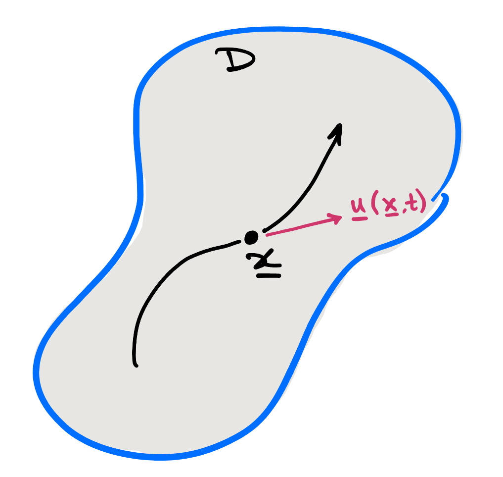
Let \(\bx\in D\) be a point in \(D\) and consider the particle of fluid that moves through the point \(\bx\) at time \(t\text{.}\) In the figure below, we sketch the trajectory that this particle might take within the fluid. Also at the point \(\bx\) at time \(t\text{,}\) we let \(\bu(\bx, t)\) be the velocity of the particle. At each fixed time, we can imagine the velocity vectors drawn at each point in the fluid; thus we call \(\bu\) the velocity field of the fluid.
At each point in space and moment in time, we assume that the fluid has a well-defined mass density, \(\rho(\bx, t)\text{.}\) Let \(V \subseteq D\) be any subregion of \(D\text{.}\) Then the mass of the fluid in \(V\) at time \(t\) is given by
In most of what follows in this chapter, we shall always assume that the functions \(\bu\text{,}\)\(\rho\text{,}\) and similarly for others describing fluid quantities are sufficiently smooth that the standard calculus operations can be applied to them. Can you think of some situations in fluid dynamics where smoothness might not be guaranteed?
The assumption that the fluid can be described by a smooth scalar density field, \(\rho\text{,}\) is a continuum assumption. This is indeed one of the core assumptions that underlies this course, but it is worth noting that this is only an assumption (albeit a widely accepted one, applicable to most real-life scenarios). On the other extreme of this view is the assumption that the fluid is composed of a discrete set of molecules, all bouncing around, and hence fluid dynamics might be posed as the study of the kinetic motion of molecules!
For example, consider the fluid density, \(\rho\text{.}\) In the continuum approximation, this needs to be a smooth mathematical function of position and time. We define it at a point \(\bx\) by taking a small volume \(\delta V\) about \(\bx\) and then define \(\rho\) as mass of the fluid particles in \(\delta V\) divided by \(\delta V\text{.}\) But how big should \(\delta V\) be? It needs to be big enough that the effects of individual particles will be smoothed out and small enough that the resulting function \(\rho\) captures macroscopic density variations in the fluid (which would be averaged out if \(\delta V\) is too large).
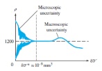
An illustration is shown in Figure 3.0.4, which shows a sketch of how the function \(\rho\) defined as particle mass in \(\delta V\) divided by \(\delta V\) might vary as \(\delta V\) varies (note the \(x\)-axis of the graph is on a logarithmic scale). The ideal choice of the volume \(\delta V\) is of the order of \(10^{-9}\) mm\(^3\) for liquids such as water, but note that the value of the density is pretty stable for a significant range around \(10^{-9}\) mm\(^3\text{,}\) and that this is necessary in order that our definition of the density makes physical sense (because the exact size of \(\delta V\) shouldn’t affect the density). For volumes much smaller than \(10^{-9}\) mm\(^3\text{,}\) we can see the effects of individual molecules. For volumes much larger, we see macroscopic effects. For liquids, a volume of \(10^{-9}\) mm\(^3\) contains about \(3\times10^7\) particles.
Figure3.0.4.Sketch illustrating how the fluid density at a point might behave, where the fluid density is defined as mass of fluid in volume \(\delta V\) divided by \(\delta V\text{,}\) and this is plotted against the volume \(\delta V\text{.}\) Note that the \(x\)-axis is on a logarithmic scale. Picture from Fig 1.2 of [8], which you can view in the University Library’s online collection
As well as the definition of the density, we need to do a similar procedure to define the velocity, and potentially other variables (pressure, stress, temperature etc). In this course, we will generally assume the procedure of choosing \(\delta V\) and averaging has already been carried out.
This approach implies there is a minimum size of the fluid body required for this approach to be valid (if we consider smaller sizes of fluid, the motion of individual particles becomes important). Specifically, a region containing about \(3\times10^7\) molecules must be small in comparison all lengthscales in the problem:
For gases at standard temperature and pressure (STP): the minimum volume is around \(10^{-18}\) m\(^3=1\)\(\mu\)m\(^3\) (this contains around \(3\times10^7\) molecules).
For liquids: the minimum volume of fluid is smaller as the particles are closer together. For water, the minimum volume is around \(10^{-21}\) m\(^3\) (this contains around \(3\times10^7\) molecules).
For complex fluids: the minimum volume needed to invoke the continuum approximation is often larger, e.g. blood contains red blood cells, which significantly affect its mechanics (the mechanics of blood plasma approximates that of water) and the volume of a single red blood cell is around \(10^{-16}\) m\(^3\text{.}\)