In this chapter, we develop the basic equations of fluid dynamics. The equations are derived from applying principles of conservation of mass and momentum. In the simplest scenario, where the fluid is assumed to be inviscid, this leads to Euler’s equations for a perfect (or ideal) fluid. Later, in Chapter 6, we relax this assumption to incorporate the effects of viscosity.
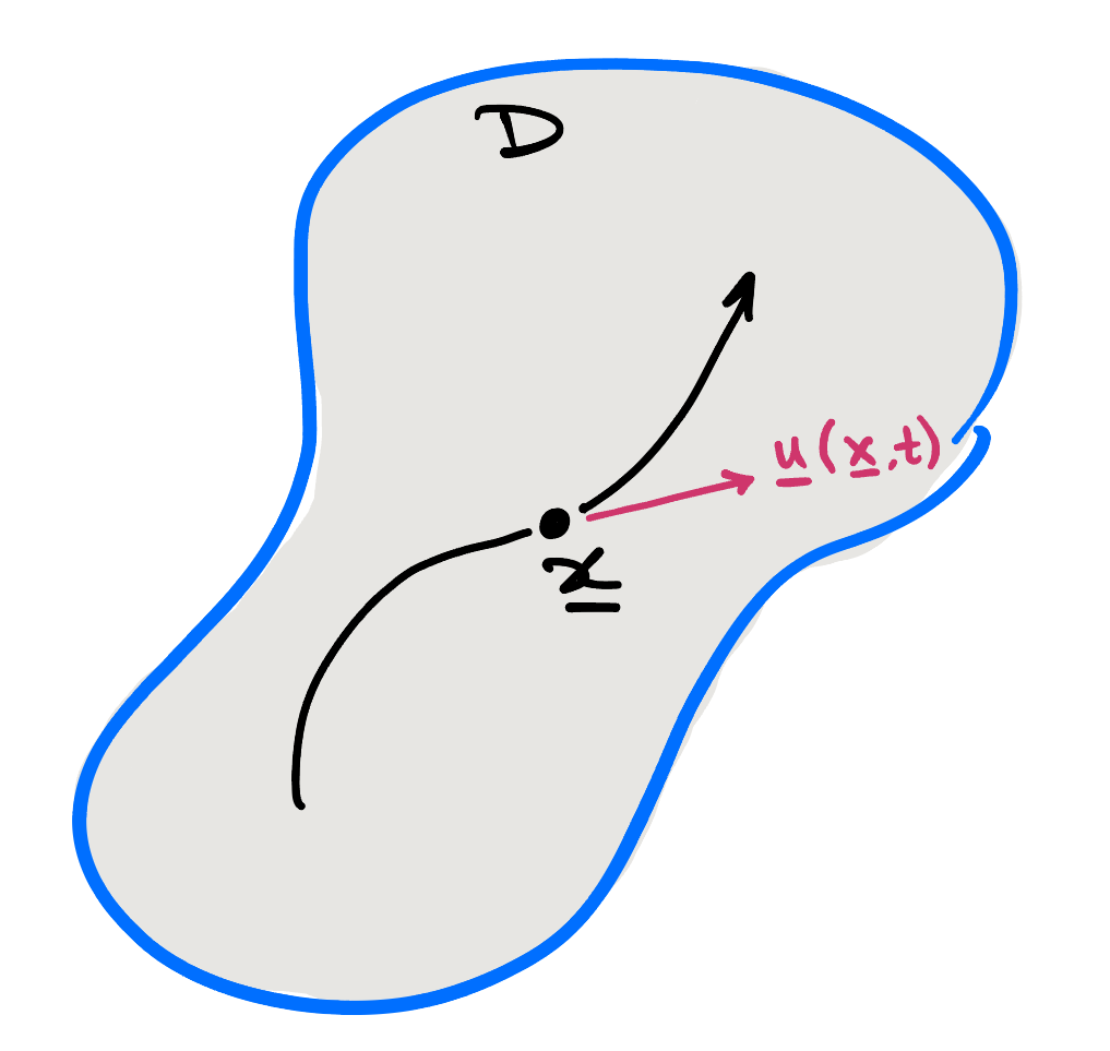
Let \(\bx\in D\) be a point in \(D\) and consider the particle of fluid that moves through the point \(\bx\) at time \(t\text{.}\) In the figure below, we sketch the trajectory that this particle might take within the fluid. Also at the point \(\bx\) at time \(t\text{,}\) we let \(\bu(\bx, t)\) be the velocity of the particle. At each fixed time, we can imagine the velocity vectors drawn at each point in the fluid; thus we call \(\bu\) the velocity field of the fluid.
At each point in space and moment in time, we assume that the fluid has a well-defined mass density, \(\rho(\bx, t)\text{.}\) Let \(V(t) \subseteq D\) be a subregion of \(D\text{,}\) possibly moving with time. Then the mass of the fluid in \(V\) at time \(t\) is given by
Throughout this chapter, we assume that \(\bu\text{,}\)\(\rho\) and the other functions describing the fluid are sufficiently smooth that the standard operations of calculus can be applied to them. Can you think of some situations in fluid dynamics where smoothness might not be guaranteed?
The assumption that the fluid can be described by a smooth scalar density field, \(\rho\text{,}\) is a continuum assumption. This is indeed one of the core assumptions that underlies this course, but it is worth noting that this is only an assumption (albeit a widely accepted one, applicable to most real-life scenarios). At the other extreme is the view that the fluid is composed of a discrete set of molecules, all bouncing around, and hence fluid dynamics might be posed as the study of the kinetic motion of molecules!