Section A.1 Kinematics

Solutions Solutions

2.3 Exercises

2.3.2. Derivation of the material derivative.

Solution.
This is the chain rule. Denote the three components of \(\bx = (x_1, x_2, x_3)\text{.}\) Then we differentiate through both outer arguments of \(f\text{:}\)
\begin{align*} \pd{f(\bx(\bX, t), t)}{t}\biggr\rvert_{\bX} &= \pd{f}{t}\biggr\rvert_{\bx} + \sum_{i=1}^3 \pd{x_i(\bX, t)}{t}\biggr\rvert_{\bX} \pd{f}{x_i} \end{align*}
The factor,
\begin{equation*} \pd{x_i}{t}\biggr\rvert_{\bX} = \dd{x_i}{t} \equiv u_i, \end{equation*}
corresponds to the velocity component in each direction. Then
\begin{equation*} \pd{f(\bx(\bX, t), t)}{t}\biggr\rvert_{\bX} = \pd{f}{t} + \bu \cdot \nabla f, \end{equation*}
as desired.
2.3.3. Eulerian and Lagrangian descriptions.

Solution.
A particle moves with the velocity of the fluid. Then it must satisfy the equations
\begin{equation*} \dd{x}{t} = -y(t),\quad \dd{y}{t} = x(t) \quad\Rightarrow\quad \dd{^2x}{t^2} = -\dd{y}{t} = -x(t). \end{equation*}
Trying solutions of the form \(x(t)=\e^{\lambda t}\) gives \(\lambda=\pm i\text{,}\) so the general solution is
\begin{equation*} x(t) = Ae^{it}+Be^{-it}, \end{equation*}
or, equivalently,
\begin{equation*} x(t) = C\cos t + D\sin t, \end{equation*}
where \(C\) and \(D\) are constants, and
\begin{equation*} y(t) =-\dd{x}{t}= C\sin t - D\cos t. \end{equation*}
Setting \(x(0)=x_0\) and \(y(0)=y_0\) gives \(C=x_0\) and \(D=-y_0\text{,}\) so
\begin{equation*} \bx(t) = (x_0\cos t - y_0\sin t, x_0\sin t + y_0\cos t). \end{equation*}
This is a circular path of radius \(\sqrt{x_0^2+y_0^2}\) going anticlockwise around the origin. The velocity is
\begin{equation*} \bu(t) = (-x_0\sin t - y_0\cos t, x_0\cos t - y_0\sin t). \end{equation*}
This flow is an example of rigid-body rotation, that is the fluid is moving with a velocity field that would be attainable for a rigid body, and there is no relative motion of the fluid particles.

2.3.4. Eulerian and Lagrangian descriptions.

2.3.4.a
Solution.
\begin{align*} \ba=&\DD{\bu}{t} \\ =& \pd{\bu}{t} + (\bu \cdot \nabla) \bu\\ =&0+\left(u\pd{u}{x}+v\pd{u}{y}+w\pd{u}{z}\right)\be_x +\left(u\pd{v}{x}+v\pd{v}{y}+w\pd{v}{z}\right)\be_y +\left(u\pd{w}{x}+v\pd{w}{y}+w\pd{w}{z}\right)\be_z\\ =& u\pd{u}{x}\be_x\\ = & U\left(1+\frac{x}{L}\right)\frac{U}{L}\be_x\\ = & \frac{U^2}{L}\left(1+\frac{x}{L}\right)\be_x \end{align*}
2.3.4.b
Solution.
We have
\begin{equation*} \dd{x}{t}=u(x)=U\left(1+\frac{x}{L}\right). \end{equation*}
Solving by separation of variables gives,
\begin{align*} &\int_0^x\frac{dx}{1+x/L}=\int_0^t U\,dt\\ \Rightarrow\quad& L\ln\left(1+\frac{x}{L}\right)=Ut\\ \Rightarrow\quad& x(t)=L\left(\e^{Ut/L}-1\right). \end{align*}
2.3.4.c
Solution.
The velocity is
\begin{align*} \dd{x}{t}=&\dd{}{t}\left(L\left(\e^{Ut/L}-1\right)\right)\\ =& L\frac{U}{L}\e^{Ut/L}\\ =& U\e^{Ut/L}. \end{align*}
2.3.4.d
Solution.
The acceleration is
\begin{align*} \dd{^2x}{t^2}=&\dd{}{t}\left(U\e^{Ut/L}\right)\\ =& \frac{U^2}{L}\e^{Ut/L}. \end{align*}
2.3.4.e
Solution.
The velocity is
\begin{equation*} U\e^{Ut/L}=U\left(1+\frac{x}{L}\right), \end{equation*}
as expected. This is the same as the Eulerian velocity at the particle position. The acceleration is
\begin{align*} \frac{U^2}{L}\e^{Ut/L}=&\frac{U^2}{L}\left(1+\frac{x}{L}\right), \end{align*}
which is the same as the particle acceleration, as expected from the definition.
2.3.4.f
Solution.
The particle reaches \(x=L\) when
\begin{align*} & L\left(\e^{Ut/L}-1\right)=L\\ \Rightarrow\quad& \e^{Ut/L}=2\\ \Rightarrow\quad& t=\frac{L}{U}\ln(2). \end{align*}

2.3.5. Particle paths and streamlines.

2.3.5.a
Solution.
Particle paths are the trajectories of individual fluid particles, which are found by solving the ODE
\begin{equation*} \dd{\bx}{t} = \bu(\bx,t). \end{equation*}
Streamlines are curves that are instantaneously tangent to the velocity field, and therefore satisfy
\begin{equation*} \dd{\bx}{s} = \bu(\bx,t), \end{equation*}
where \(s\) is a parameter along the streamline. The two coincide if the flow is steady, i.e. \(\bu(\bx,t)=\bu(\bx)\text{.}\)
2.3.5.b
Solution.
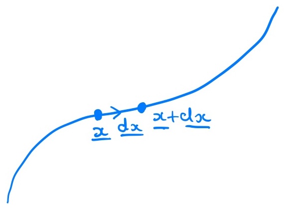
Figure 2.10. Pathline, showing the particle positions at times \(t\) and \(t+\de t\text{.}\)
Figure 2.10 shows the particle at \(\bx = \bx(t)\) and at \(\bx(t + \de t) = \bx + \de\bx\text{.}\) Since the curve is a pathline, \(\de\bx = \bu(\bx, t) \, \de t + O(\de t^2)\text{;}\) in particular, \(|\de\bx| = O(\de t)\text{,}\) so all of the remainder terms in the Taylor series are \(O(\de t^2)\text{.}\) Following the value of \(f\) along the pathline,
\begin{align*} \dd{F}{t} &= \lim_{\de t \to 0} \frac{1}{\de t} \Big( f(\bx + \de\bx, t + \de t) - f(\bx, t) \Big)\\ &= \lim_{\de t \to 0} \frac{1}{\de t} \Big( \de\bx \cdot \nabla f(\bx, t) + \de t \, \pd{f}{t}(\bx, t) + O(\de t^2) \Big)\\ &= \lim_{\de t \to 0} \frac{1}{\de t} \Big( \de t \, \bu(\bx, t) \cdot \nabla f(\bx, t) + \de t \, \pd{f}{t}(\bx, t) + O(\de t^2) \Big)\\ &= \pd{f}{t} + \bu \cdot \nabla f = \DD{f}{t}. \end{align*}
The value of \(f\) carried by the particle, \(F(t)\text{,}\) is constant for all \(t\) if and only if \(\dd{F}{t} = 0\text{.}\) Since this holds for every pathline, \(f\) is preserved following the flow if and only if \(\DD{f}{t} = 0\text{.}\)
2.3.5.c
Solution.
The two points \(\bx = \bx(s, t)\) and \(\bx + \de\bx = \bx(s + \de s, t)\) lie on the same streamline at the same time, and could be sketched as in Figure 2.10, with the parameter \(s\) in place of \(t\text{.}\) Since the curve is a streamline, \(\de\bx = \bu(\bx, t) \, \de s + O(\de s^2)\text{,}\) so \(|\de\bx| = O(\de s)\text{.}\) Following the value of \(f\) along the streamline,
\begin{align*} \dd{G}{s} &= \lim_{\de s \to 0} \frac{1}{\de s} \Big( f(\bx + \de\bx, t) - f(\bx, t) \Big)\\ &= \lim_{\de s \to 0} \frac{1}{\de s} \Big( \de\bx \cdot \nabla f(\bx, t) + O(\de s^2) \Big)\\ &= \lim_{\de s \to 0} \frac{1}{\de s} \Big( \de s \, \bu(\bx, t) \cdot \nabla f(\bx, t) + O(\de s^2) \Big)\\ &= \bu \cdot \nabla f. \end{align*}
Hence \(G(s)\) is constant along the streamline if and only if \(\bu \cdot \nabla f = 0\text{.}\) Compared with the previous part, time is frozen here, so there is no \(\pd{f}{t}\) term. If both the flow and \(f\) are steady, then the streamlines and pathlines coincide (see the first part) and \(\DD{f}{t} = \bu \cdot \nabla f\text{,}\) so the two conditions are the same.

2.3.6. Streamlines, pathlines and streaklines.

2.3.6.a
Solution.
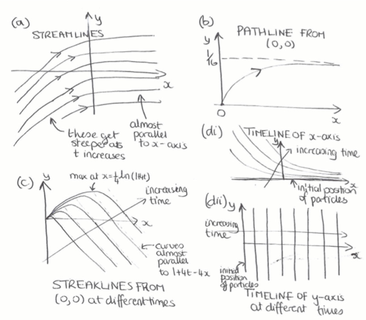
The streamlines are given by
\begin{equation*} \pd{y}{x}=te^{-4x}\quad\Rightarrow\quad y=y_0-\frac{t}{4} e^{-4x}, \end{equation*}
for any constant \(y_0\text{.}\) Different values of \(y_0\) give different streamlines. See Figure 2.11 for a sketch.
Figure 2.11. Sketch of streamlines, pathline and streaklines.
2.3.6.b
Solution.
The pathlines for a particle starting from \((x_0,y_0)\) are given by
\begin{align*} &\dd{x}{t}=1,\quad \dd{y}{t}=te^{-4x}\\ \Rightarrow\quad& x = x_0 + t,\quad y = y_0 + \frac{1}{16} e^{-4x_0} - \frac{1+4t}{16} e^{-4(x_0+t)}. \end{align*}
Eliminating \(t\text{:}\)
\begin{equation*} y = y_0 + \frac{1}{16} e^{-4x_0} - \frac{1+4x-4x_0}{16} e^{-4x}. \end{equation*}
This is a general pathline. For the particular particle that starts from \((0,0)\text{:}\)
\begin{equation*} y = \tfrac{1}{16}\left(1 - (1+4x)e^{-4x}\right). \end{equation*}
See Figure 2.11 for a sketch.
2.3.6.c
Solution.
Suppose the particle that started at \((x_0,y_0)\) hits the special point \((0,0)\) at time \(t_1\text{.}\) From the pathline equation:
\begin{equation*} 0 = x_0 + t_1, \quad 0 = y_0 + \tfrac{1}{16} e^{-4x_0} - \tfrac{1+4t_1}{16} e^{-4(x_0+t_1)}. \end{equation*}
Solving for \(x_0\) and \(y_0\text{:}\)
\begin{equation*} x_0 = -t_1,\quad y_0 = -\tfrac{1}{16}\left(e^{4t_1} - 1 - 4t_1\right). \end{equation*}
At time \(t\) the particle is at:
\begin{equation*} x = t - t_1,\quad y = \tfrac{1}{16}\left((1+4t_1) - (1+4t)e^{-4(t-t_1)}\right). \end{equation*}
Eliminating \(t_1\) gives the streakline at time \(t\text{:}\)
\begin{equation*} y = \tfrac{1}{16}\left((1+4t)(1-e^{-4x}) - 4x\right). \end{equation*}
See Figure 2.11 for a sketch. Note that the streamlines, pathlines and streaklines are all very different.
2.3.6.d
Solution.
From the pathline equation, a particle starting from \((x_0,0)\) reaches
\begin{equation*} x = x_0 + t,\quad y = \tfrac{1}{16} e^{-4x_0} - \tfrac{1+4t}{16} e^{-4(x_0+t)} \end{equation*}
at time \(t\text{.}\) Eliminating \(x_0\) gives the timeline:
\begin{equation*} y = \tfrac{1}{16}\left(e^{4t} - 1 - 4t\right)e^{-4x}. \end{equation*}
See Figure 2.11 for a sketch.
From the pathline equation, a particle starting from \((0,y_0)\) reaches
\begin{equation*} x = t,\quad y = y_0 + \tfrac{1}{16} - \tfrac{1+4t}{16} e^{-4t} \end{equation*}
at time \(t\text{.}\) Since \(y_0\) can take any value, the timeline is just the line \(x = t\text{.}\) See Figure 2.11 for a sketch.