Section A.2 Equations of motion

Solutions Solutions

3.6 Exercises

3.6.1. Bump lemma.

Solution.
This proof assumes that the function \(f\) is not pathological (e.g. it cannot oscillate infinitely fast, take different values for rational vs. irrational, etc.). That’s what we mean by "sufficiently smooth".
Assume that there exists a point \(\bx_0 \in \Omega\) where \(f(\bx_0) \neq 0\text{.}\) Suppose without loss of generality \(f > 0\) here. Since \(f\) is sufficiently smooth (and in particular, it is continuous), then there exists a non-trivial neighbourhood of \(\bx_0\text{,}\) say \(V_0\text{,}\) where \(f > 0\) everywhere. Then \(\int_{V_0} f \, \de{V} > 0\text{,}\) contradicting the assumption. Therefore \(f\) must be zero everywhere.

3.6.2. Leibniz’s rule.

3.6.2.a
Solution.
The first circled element is associated with the quantity:
\begin{equation*} \frac{1}{\Delta t} \int_{a(t)}^{b(t)} [f(x, t + \Delta t) - f(x, t)] \, \de{x}. \end{equation*}
This is essentially the finite-difference version of the first term on the RHS.
The second circled element is associated with the quantity:
\begin{equation*} -f(a(t), t)[a(t + \Delta t) - a(t)] \frac{1}{\Delta t}. \end{equation*}
This is the area of the left-hand (blue) rectangle, which is lost from the integral as the lower limit moves to the right, hence the minus sign.
The third circled element is associated with
\begin{equation*} f(b(t), t + \Delta t)[b(t + \Delta t) - b(t)] \frac{1}{\Delta t}. \end{equation*}
This is the area of the right-hand (pink) rectangle, which is gained as the upper limit moves to the right. Notice that for small \(\Delta t\text{,}\) the rectangle height \(f(b, t+\Delta t)\) is approximately \(f(b, t)\text{.}\)
3.6.2.b
Solution.
Let \(I(t) = \int_{a(t)}^{b(t)} f(x, t) \, \de{x}\text{.}\) Splitting the range of integration,
\begin{align*} I(t + \Delta t) &= \int_{a(t + \Delta t)}^{b(t + \Delta t)} f(x, t + \Delta t) \, \de{x}\\ &= \int_{a(t)}^{b(t)} f(x, t + \Delta t) \, \de{x} + \int_{b(t)}^{b(t + \Delta t)} f(x, t + \Delta t) \, \de{x}\\ &\quad - \int_{a(t)}^{a(t + \Delta t)} f(x, t + \Delta t) \, \de{x}. \end{align*}
Subtracting \(I(t)\) and dividing by \(\Delta t\) gives
\begin{align*} \frac{I(t + \Delta t) - I(t)}{\Delta t} &= \int_{a(t)}^{b(t)} \frac{f(x, t + \Delta t) - f(x, t)}{\Delta t} \, \de{x}\\ &\quad + \frac{1}{\Delta t}\int_{b(t)}^{b(t + \Delta t)} f(x, t + \Delta t) \, \de{x}\\ &\quad - \frac{1}{\Delta t}\int_{a(t)}^{a(t + \Delta t)} f(x, t + \Delta t) \, \de{x}. \end{align*}
These three terms correspond to the circled regions 1, 3 and 2 of Figure 3.5 respectively. We take the limit \(\Delta t \to 0\) in each.
First term. For small \(\Delta t\text{,}\) the integrand is the difference quotient of \(f\) in time, which is approximately \(\pd{f}{t}\text{.}\) Since \(\pd{f}{t}\) is continuous, this approximation improves uniformly across the interval as \(\Delta t \to 0\text{,}\) and the first term tends to
\begin{equation*} \int_{a(t)}^{b(t)} \pd{f}{t} \, \de{x}. \end{equation*}
Second term. For small \(\Delta t\text{,}\) the interval from \(b(t)\) to \(b(t + \Delta t)\) is narrow, with width approximately \(\dot{b}\,\Delta t\text{,}\) and across it \(f(x, t + \Delta t)\) is close to \(f(b(t), t)\text{.}\) We may therefore approximate the integral by the area of a single rectangle (a one-term Riemann sum):
\begin{equation*} \frac{1}{\Delta t}\int_{b(t)}^{b(t + \Delta t)} f(x, t + \Delta t) \, \de{x} \approx f(b(t), t) \, \frac{b(t + \Delta t) - b(t)}{\Delta t}. \end{equation*}
Since \(f\) is continuous, the error in this approximation is small compared with \(\Delta t\text{,}\) and so disappears in the limit. The term therefore tends to \(f(b(t), t)\,\dot{b}(t)\text{.}\)
Third term. In the same way, this tends to \(-f(a(t), t)\,\dot{a}(t)\text{.}\)
Adding the three limits gives Leibniz’s rule (3.6.1).
3.6.2.c
Solution.
In one dimension, with \(a(t)\) and \(b(t)\) moving with the fluid (so \(\dot{a} = u(a, t)\) and \(\dot{b} = u(b, t)\)), Reynolds’ Transport Theorem reads
\begin{equation*} \dd{}{t} \int_{a(t)}^{b(t)} f \, \de{x} = \int_{a(t)}^{b(t)} \left[ \pd{f}{t} + \pd{}{x}(f u) \right] \de{x}. \end{equation*}
Integrating the second term gives
\begin{equation*} f(b, t)u(b, t) - f(a, t)u(a, t) = f(b, t)\dot{b} - f(a, t)\dot{a}, \end{equation*}
which are exactly the second and third terms of Leibniz’s rule.

3.6.3. Derivation of governing equations.

Solution.
The proof of the continuity equation is given in Theorem 3.2.1 and the proof of the momentum equation is given in Theorem 3.3.1, so make sure you can follow these arguments and produce your own notes.
The derivation of the Euler equations, as given in Definition 3.4.5 requires the additional assumption of an incompressible fluid of constant density, following Theorem 3.4.1. Incompressibility implies that \(\nabla \cdot \bu = 0\text{,}\) and this equation then replaces the continuity equation.

3.6.4. Pressure field in uniform flow.

3.6.4.a
Solution.
The fluid has a uniform velocity, which means that all components of \(\nabla\bu\) vanish. The Euler equation simplifies to
\begin{equation*} \rho\pd{\bu}{t}=-\nabla p-\rho g \bk, \end{equation*}
where
\begin{equation*} \pd{\bu}{t}=(b, \; 3t^2, \; \e^t). \end{equation*}
Hence, the pressure is given by solving the equation,
\begin{equation*} \nabla p = -\rho \pd{\bu}{t} - \rho g \bk = -\rho (\, b, \; 3t^2, \; \e^t + g \,), \end{equation*}
which is a vector equation. Splitting into components, we obtain
\begin{equation*} \frac{\partial p}{\partial x} = -\rho b, \quad \frac{\partial p}{\partial y} = -3\rho t^2, \quad \frac{\partial p}{\partial z} = -\rho (\e^t + g). \end{equation*}
Solving sequentially, the first equation gives
\begin{equation*} p = -\rho b x + f_1(y,z,t). \end{equation*}
Substituting into the second equation,
\begin{equation*} \frac{\partial f_1}{\partial y} = -3\rho t^2 \;\;\Rightarrow\;\; f_1 = -3\rho t^2 y + f_2(z,t), \end{equation*}
\begin{equation*} p = -\rho b x - 3\rho t^2 y + f_2(z,t). \end{equation*}
The third equation then implies
\begin{equation*} \frac{\partial f_2}{\partial z} = -\rho(\e^t+g) \;\;\Rightarrow\;\; f_2 = -\rho(\e^t+g)z + f_3(t), \end{equation*}
\begin{equation*} p = -\rho b x - 3\rho t^2 y - \rho(\e^t+g)z + f_3(t). \end{equation*}
Using \(p = p_0\) at the origin gives \(f_3(t) = p_0\) for all \(t\text{.}\) Hence
\begin{equation*} p = p_0 - \rho \big(bx + 3t^2 y + (\e^t + g)z \big). \end{equation*}

3.6.4.b
Solution.
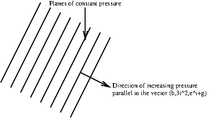
The pressure is constant on parallel planes normal to the vector \((b, \; 3t^2, \; \e^t + g)\text{,}\) as illustrated below:
Figure 3.6. Contours of the pressure field at fixed \(t\text{.}\)

3.6.5. Piston problem.

Solution.
We assume that the fluid pressure at the open end of the pipe is atmospheric pressure. Since the fluid moves as a rigid body, the velocity field has no spatial gradients, and hence the Euler equation reduces to
\begin{equation*} \rho\pd{\bu}{t}=-\nabla p, \end{equation*}
where the velocity is uniformly \(\bu=(\dot{X}(t),0)\text{.}\)
Solving for \(p\) and using the fact that \(p\) is atmospheric pressure at \(x = L\text{,}\) we have
\begin{equation*} p(x,t) = \rho\dd{^2 X}{t^2}(L-x)+p_\text{atm}. \end{equation*}
At the piston \(x=X\text{,}\) note that atmospheric pressure applies in addition to \(F\text{,}\) meaning that the force on the fluid is
\begin{equation*} F+Ap_\text{atm}, \end{equation*}
and hence the fluid pressure is
\begin{equation*} \frac{F}{A} + p_\text{atm}. \end{equation*}
Then
\begin{equation*} \frac{F}{A} + p_\text{atm} = \rho\dd{^2X}{t^2}(L-X)+p_\text{atm} \quad\Rightarrow\quad \dd{^2X}{t^2} = \frac{F}{A\rho(L-X)}. \end{equation*}
Note that the atmospheric pressure cancels in this problem, and this is common to problems of this type, because atmospheric pressure acts uniformly on all surfaces exposed to the atmosphere and therefore does not lead to a resultant force or affect the dynamics. This motivates the introduction of a gauge pressure, \(p_{\text{gauge}}\text{,}\) whereby a uniform and constant baseline pressure is chosen, in this case \(p_{\text{atm}}\text{,}\) with the gauge pressure given by \(p_{\text{gauge}}=p-p_{\text{atm}}\text{.}\) Since the pressure only appears as a gradient in the governing equations, using the gauge pressure does not affect the result. Introducing a gauge pressure can make the algebra simpler.

3.6.6. Using streamlines: The clepsydra.

3.6.6.a
Solution.
The fluid velocity at the surface of the jar satisfies \(\bu\cdot\bn=0\text{,}\) so that no fluid leaves or enters the jar through its sides. This means that the flow next to the boundary of the jar must be parallel to this boundary, meaning that streamlines are parallel to the boundary. Equivalently, the boundary \(r = a(z)\) is a streamline.
3.6.6.b
Solution.
We apply Bernoulli’s equation to equate the energy at a point at the edge of the free surface at \(z = h(t)\) and the fluid leaving the hole at \(z = 0\text{.}\) At the free surface, the pressure is atmospheric, \(p = p_\text{atm}\text{,}\) and the speed is \(u_S\sqrt{1+a^{'2}}\text{.}\) At the hole, the pressure is also atmospheric, \(p = p_\text{atm}\text{,}\) and the velocity is \(u\text{.}\) Thus, Bernoulli’s equation for the streamline joining the two points gives
\begin{equation*} \frac{p_\text{atm}}{\rho} + \frac12 u_S^2(1+a^{'2}) + gh = \frac{p_\text{atm}}{\rho} + \frac12 u^2. \end{equation*}
Assuming that \(u_S \ll u\text{,}\) this simplifies to
\begin{equation*} gh = \frac12 u^2. \end{equation*}
3.6.6.c
Solution.
The volume flux out of the hole is \(\pi a_h^2 u\text{,}\) while the rate of decrease of the volume of fluid in the jar is \(\pi a(h(t))^2 u_S\text{.}\) Conservation of mass therefore gives
\begin{equation*} \pi a^2 u_S = \pi a_h^2 u, \end{equation*}
or
\begin{equation*} u_S = \frac{a_h^2}{a^2}u. \end{equation*}
Using the result from part (b) to eliminate \(u\) gives
\begin{equation*} u_S = \frac{a_h^2}{a^2}\sqrt{2gh}. \end{equation*}
We require \(u_S\) to be independent of time so that equally spaced intervals are traversed in equal times. Hence,
\begin{equation*} a=\left(\frac{a_h^2\sqrt{2g}}{u_S}\right)^{1/2} h^{1/4}. \end{equation*}
The terms in the brackets are constant, so we have that the radius of the jar must vary as the fourth root of the height.

3.6.7. Verifying Reynolds’ Transport Theorem.

3.6.7.a
Solution.
Integrating over \(V(t)\text{,}\)
\begin{align*} I(t) &= \int_0^1 \int_0^{\e^{-t/2}} \int_0^{\e^{t}} (x^2 + y) \, \de{x} \, \de{y} \, \de{z}\\ &= \underbrace{\frac{\e^{3t}}{3} \cdot \e^{-t/2}}_{x^2 \text{ term}} + \underbrace{\e^{t} \cdot \frac{\e^{-t}}{2}}_{y \text{ term}} = \frac13 \e^{5t/2} + \frac12. \end{align*}
Therefore
\begin{equation*} \dd{I}{t} = \frac56 \e^{5t/2}. \end{equation*}
3.6.7.b
Solution.
Here \(\pd{f}{t} = 0\) and
\begin{equation*} f\bu = \left( (x^2 + y)x, \; -\tfrac12 (x^2 + y)y, \; 0 \right), \end{equation*}
so
\begin{equation*} \nabla \cdot (f\bu) = (3x^2 + y) - \tfrac12 (x^2 + 2y) = \tfrac52 x^2. \end{equation*}
Hence
\begin{align*} \iiint_{V(t)} \left[ \pd{f}{t} + \nabla \cdot (f\bu) \right] \de{x} \, \de{y} \, \de{z} &= \frac52 \int_0^1 \int_0^{\e^{-t/2}} \int_0^{\e^{t}} x^2 \, \de{x} \, \de{y} \, \de{z}\\ &= \frac52 \cdot \frac{\e^{3t}}{3} \cdot \e^{-t/2} = \frac56 \e^{5t/2}, \end{align*}
in agreement with the previous part.
As a check, we can also follow the Lagrangian route used in the proof of Theorem 3.1.3. Mapping back to the fixed cube \(V(0)\text{,}\)
\begin{align*} I(t) &= \iiint_{V(0)} f\big(\bx(\bX, t)\big) \, J \, \de{X} \, \de{Y} \, \de{Z}\\ &= \int_0^1 \int_0^1 \int_0^1 \left( X^2 \e^{2t} + Y \e^{-t/2} \right) \e^{t/2} \, \de{X} \, \de{Y} \, \de{Z}\\ &= \frac13 \e^{5t/2} + \frac12, \end{align*}
which is now an integral over a fixed domain, so the time derivative can be taken inside the integral.

3.6.8. Measuring airspeed with a Pitot tube.

3.6.8.a
Solution.
The tube is sealed at its far end by the water in the manometer, so once the water has settled, no air flows into the tube. The air arriving at the tip must therefore come to rest there: the tip is a stagnation point.
The flow is steady and inviscid, so Theorem 3.5.7 applies along the streamline that runs from far upstream to the tip. Far upstream the pressure is \(p_\infty\) and the speed is \(U\text{;}\) at the tip the pressure is \(p_0\) and the speed is zero. Changes in height along the streamline are small, so the gravity terms cancel. Hence
\begin{equation*} \frac{p_\infty}{\rho_\text{air}} + \frac12 U^2 = \frac{p_0}{\rho_\text{air}}, \end{equation*}
which gives
\begin{equation*} p_0 = p_\infty + \frac12 \rho_\text{air} U^2. \end{equation*}
The pressure \(p_0\) is called the stagnation pressure.
3.6.8.b
Solution.
The water is at rest, so from Example 3.5.12 the quantity \(p + \rho_w g z\) is the same everywhere in the water. The water surface in the arm connected to the Pitot tube is at \(z = h_1\text{,}\) where the pressure is \(p_0\text{,}\) and the surface in the open arm is at \(z = h_2\text{,}\) where the pressure is \(p_\infty\text{.}\) Then
\begin{equation*} p_0 + \rho_w g h_1 = p_\infty + \rho_w g h_2, \end{equation*}
so that \(p_0 - p_\infty = \rho_w g (h_2 - h_1) = \rho_w g \Delta h\text{.}\)
3.6.8.c
Solution.
Combining the two previous parts,
\begin{equation*} \frac12 \rho_\text{air} U^2 = p_0 - p_\infty = \rho_w g \Delta h, \end{equation*}
and so
\begin{equation*} U = \sqrt{\frac{2 \rho_w g \Delta h}{\rho_\text{air}}}. \end{equation*}
With the given values, \(\Delta h = 0.75 - 0.25 = 0.5\) m, so
\begin{equation*} p_0 - p_\infty = 1000 \times 10 \times 0.5 = 5000 \text{ Pa}, \qquad U^2 = \frac{2 \times 5000}{1} = 10^4 \text{ m}^2/\text{s}^2, \end{equation*}
so \(U = 100\) m/s, or \(360\) km/h. This is roughly the take-off speed of a passenger jet.