Section A.3 Potential flows

Solutions Solutions

4.7 Exercises

4.7.1. Basic calculations.

4.7.1.a

Solution.

(i) From Example 4.1.2 and Subsection 4.3.2, with \(\alpha = \pi/4\text{,}\)

\begin{equation*} f(z) = U\e^{-\im\alpha}z = U\e^{-\im \pi/4}z. \end{equation*}

(ii) The complex velocity is \(f'(z) = u - \im v = U\e^{-\im \pi/4}\text{,}\) so

\begin{equation*} \bu = U \Bigl[ \cos(\pi/4), \, \sin(\pi/4) \Bigr] = \frac{U}{\sqrt{2}} [1, 1]. \end{equation*}

(iii) We expect the flux through the circle to be zero, since as much fluid enters one side as leaves the other. With \(\bn = [\cos\theta, \sin\theta]\) and \(\de{s} = \de\theta\text{,}\)

\begin{equation*} \int_{r = 1} \bu \cdot \bn \, \de{s} = \frac{U}{\sqrt{2}} \int_0^{2\pi} (\cos\theta + \sin\theta) \, \de{\theta} = 0. \end{equation*}

(iv) Parametrising the plate by \(\br(t) = [t, 1 - t]\text{,}\) \(0 \leq t \leq 1\text{,}\) the tangent is \(\br'(t) = [1, -1]\text{,}\) so the unit normal pointing away from the origin is

\begin{equation*} \bn = \frac{[1, 1]}{\sqrt{2}}, \end{equation*}

and \(\de{s} = |\br'(t)| \, \de{t} = \sqrt{2} \, \de{t}\text{.}\) The flux is then

\begin{equation*} \int_0^1 \frac{U}{\sqrt{2}} [1, 1] \cdot \frac{[1, 1]}{\sqrt{2}} \, \sqrt{2} \, \de{t} = \sqrt{2}\,U. \end{equation*}

This makes sense: the flow is everywhere normal to the plate, with speed \(U\text{,}\) and the plate has length \(\sqrt{2}\text{.}\)

4.7.1.b

Solution.

(i) From (4.3.5),

\begin{equation*} f(z) = \frac{Q}{2\pi}\log z. \end{equation*}

(ii) The complex velocity is

\begin{align*} u - \im v = f'(z) \amp= \frac{Q}{2\pi z} = \frac{Q}{2\pi r}\e^{-\im\theta}\\ \amp= \frac{Q}{2\pi r}(\cos\theta - \im\sin\theta), \end{align*}

\begin{equation*} \bu = \frac{Q}{2\pi r}[\cos\theta, \sin\theta] = \frac{Q}{2\pi}\frac{[x, y]}{x^2 + y^2}. \end{equation*}

(iii) On the unit circle, \(r = 1\text{,}\) \(\bn = [\cos\theta, \sin\theta]\) and \(\de{s} = \de\theta\text{,}\) so

\begin{align*} \int_{r = 1} \bu \cdot \bn \, \de{s} \amp= \int_0^{2\pi} \frac{Q}{2\pi} [\cos\theta, \sin\theta] \cdot [\cos\theta, \sin\theta] \, \de\theta\\ \amp= \frac{Q}{2\pi}\int_0^{2\pi} \de\theta = Q. \end{align*}

This is the definition of the source strength: all of the fluid produced at the origin crosses the circle.

(iv) As in part (a), parametrise the plate by \(\br(t) = [t, 1 - t]\text{,}\) \(0 \leq t \leq 1\text{,}\) with \(\bn = [1, 1]/\sqrt{2}\) and \(\de{s} = \sqrt{2}\,\de{t}\text{.}\) On the plate, \(x = t\) and \(y = 1 - t\text{,}\) so \(x + y = 1\) and \(x^2 + y^2 = t^2 + (1 - t)^2\text{.}\) Hence

\begin{align*} \textrm{flux} \amp= \int_0^1 \frac{Q}{2\pi}\frac{[x, y]}{x^2 + y^2} \cdot \frac{[1, 1]}{\sqrt{2}} \, \sqrt{2}\,\de{t}\\ \amp= \frac{Q}{2\pi}\int_0^1 \frac{x + y}{x^2 + y^2}\,\de{t}\\ \amp= \frac{Q}{2\pi}\int_0^1 \frac{\de{t}}{t^2 + (1 - t)^2}\\ \amp= \frac{Q}{2\pi}\cdot\frac{\pi}{2} = \frac{Q}{4}. \end{align*}

This makes sense: the source sends fluid out equally in all directions, and the plate spans a quarter of the directions seen from the origin (from \(\theta = 0\) to \(\theta = \pi/2\)), so it receives a quarter of the flux. In Exercise 4.7.2, you will see that this follows immediately from the streamfunction, \(\psi = Q\theta/(2\pi)\text{.}\)

4.7.1.c

Solution.

(i) From Subsection 4.3.2,

\begin{equation*} f(z) = \frac{z^2}{2}. \end{equation*}

(ii) The complex velocity is \(f'(z) = z = x + \im y = u - \im v\text{,}\) so

\begin{equation*} \bu = [x, -y]. \end{equation*}

(iii) On the unit circle, \([x, y] = [\cos\theta, \sin\theta]\text{,}\) \(\bn = [\cos\theta, \sin\theta]\) and \(\de{s} = \de\theta\text{,}\) so

\begin{align*} \int_{r = 1} \bu \cdot \bn \, \de{s} \amp= \int_0^{2\pi} [\cos\theta, -\sin\theta] \cdot [\cos\theta, \sin\theta] \, \de\theta\\ \amp= \int_0^{2\pi} (\cos^2\theta - \sin^2\theta) \, \de\theta = \int_0^{2\pi} \cos 2\theta \, \de\theta = 0. \end{align*}

Fluid enters the circle near the \(y\)-axis and leaves near the \(x\)-axis, with no net flux.

\begin{align*} \textrm{flux} \amp= \int_0^1 [t, -(1 - t)] \cdot \frac{[1, 1]}{\sqrt{2}} \, \sqrt{2}\,\de{t}\\ \amp= \int_0^1 (2t - 1) \, \de{t} = \Bigl[t^2 - t\Bigr]_0^1 = 0. \end{align*}

This is consistent with Theorem 4.2.2: the streamfunction \(\psi = xy\) is zero at both ends of the plate, \((0, 1)\) and \((1, 0)\text{.}\)

4.7.1.d

Solution.

(i) From (4.3.7),

\begin{equation*} f(z) = -\frac{\im\Gamma}{2\pi}\log z. \end{equation*}

(ii) The complex velocity is

\begin{align*} u - \im v = f'(z) \amp= -\frac{\im\Gamma}{2\pi z} = -\frac{\im\Gamma}{2\pi r}(\cos\theta - \im\sin\theta)\\ \amp= \frac{\Gamma}{2\pi r}(-\sin\theta - \im\cos\theta), \end{align*}

\begin{equation*} \bu = \frac{\Gamma}{2\pi r}[-\sin\theta, \cos\theta] = \frac{\Gamma}{2\pi}\frac{[-y, x]}{x^2 + y^2}. \end{equation*}

(iii) On the unit circle, \(\bn = [\cos\theta, \sin\theta]\) and \(\de{s} = \de\theta\text{,}\) so

\begin{align*} \int_{r = 1} \bu \cdot \bn \, \de{s} \amp= \frac{\Gamma}{2\pi}\int_0^{2\pi} [-\sin\theta, \cos\theta] \cdot [\cos\theta, \sin\theta] \, \de\theta\\ \amp= 0. \end{align*}

The integrand is zero: the flow is everywhere tangent to the circle, so no fluid crosses it.

(iv) As in part (a), parametrise the plate by \(\br(t) = [t, 1 - t]\text{,}\) \(0 \leq t \leq 1\text{,}\) with \(\bn = [1, 1]/\sqrt{2}\) and \(\de{s} = \sqrt{2}\,\de{t}\text{.}\) On the plate, \(-y + x = 2t - 1\) and \(x^2 + y^2 = t^2 + (1 - t)^2\text{,}\) so

\begin{align*} \textrm{flux} \amp= \int_0^1 \frac{\Gamma}{2\pi}\frac{[-y, x]}{x^2 + y^2} \cdot \frac{[1, 1]}{\sqrt{2}} \, \sqrt{2}\,\de{t}\\ \amp= \frac{\Gamma}{2\pi}\int_0^1 \frac{2t - 1}{t^2 + (1 - t)^2}\,\de{t}. \end{align*}

The denominator is \(2t^2 - 2t + 1\text{,}\) whose derivative is \(2(2t - 1)\text{,}\) so

\begin{equation*} \textrm{flux} = \frac{\Gamma}{4\pi}\Bigl[\log(2t^2 - 2t + 1)\Bigr]_0^1 = \frac{\Gamma}{4\pi}(\log 1 - \log 1) = 0. \end{equation*}

Alternatively, under \(t \mapsto 1 - t\) the numerator changes sign while the denominator is unchanged, so the integral is zero. This is consistent with Theorem 4.2.2: the streamfunction \(\psi = -(\Gamma/2\pi)\log r\) takes the same value at both ends of the plate, which are both at distance \(r = 1\) from the origin.

4.7.2. Evaluation of the flux.

Solution.

This is a nice question to do because there is a simple recipe. For each of the complex potentials in the previous question, find the imaginary part to obtain the streamfunction. Then evaluate the difference in streamfunction values at the start and end values of the desired curve.

For uniform flow, \(\psi(r, \theta) = Ur \sin(\theta - \alpha)|\text{.}\) For the case of a circle, the flux is:

\begin{equation*} |\psi(1, 2\pi) - \psi(1, 0)| = 0. \end{equation*}

For the case of a plate,

\begin{equation*} |\psi(1, 0) - \psi(1, \pi/2)| = U|\sin(-\pi/4) - \sin(\pi/4)| = \sqrt{2}U. \end{equation*}

For source flow, \(\psi = (Q/2\pi) \theta\) once you convert the logarithm into its real and complex parts. Then for the circle:

\begin{equation*} |\psi(1, 2\pi) - \psi(1, 0)| = Q. \end{equation*}

For the case of the plate,

\begin{equation*} |\psi(1, 0) - \psi(1, \pi/2)| = \frac{Q}{4}. \end{equation*}

(Actually calculating the above might convince you the route of calculating flux by integrals is possible!).

For the stagnation point, \(\psi = (r^2/2)\sin 2\theta\text{.}\) For the circle,

\begin{equation*} |\psi(1, 2\pi) - \psi(1, 0)| = 0. \end{equation*}

For the case of the plate,

\begin{equation*} |\psi(1, 0) - \psi(1, \pi/2)| = 0. \end{equation*}

For the case of the line vortex, \(\psi = -\Gamma/(2\pi)\log r\text{,}\) and for the circle,

\begin{equation*} |\psi(1, 2\pi) - \psi(1, 0)| = 0, \end{equation*}

while for the plate,

\begin{equation*} |\psi(1, 0) - \psi(1, \pi/2)| = 0. \end{equation*}

4.7.3. Doublet.

4.7.3.a

Solution.

The complex potential is the sum of a line source and line sink:

\begin{equation*} f(z) = \frac{Q}{2\pi} [\log(z - a) - \log(z + a)]. \end{equation*}

Therefore the complex velocity is given by

\begin{equation*} f'(z) = \frac{Q}{2\pi} \left[ \frac{1}{z-a} - \frac{1}{z+a}\right]. \end{equation*}

Stagnation points are where \(f'(z) = 0\text{.}\) There are no stagnation points. The streamfunction is given by

\begin{equation*} \Im f = \frac{Q}{2\pi}(\theta_1 - \theta_2), \end{equation*}

where \(\theta_1\) and \(\theta_2\) are angles measured relative to the positions about \(\pm a\text{.}\) Thus,

\begin{equation*} \theta_{1,2} = \tan^{-1} \left( \frac{y}{x \mp a} \right). \end{equation*}

The streamlines are given where \(\psi\) is constant. The streamlines are shown below.

Almost doublet — Figure 4.19. Streamlines for a sink and source

4.7.3.b

Solution.

Expanding the logarithms for small \(a\) gives

\begin{equation*} \log z - \log z + \log(1 - a/z) - \log(1 + a/z) \sim -\frac{2a}{z}. \end{equation*}

Thus in the limit \(a \to 0\text{,}\) we have

\begin{equation*} f(z) \sim -\frac{Qa}{\pi} \frac{1}{z}. \end{equation*}

Therefore, we let both \(a \to 0\) and \(Q \to \infty\) in a fashion such that \(m = aQ\) is fixed. We then have the potential

\begin{equation*} f(z) = \frac{\mu}{z} \end{equation*}

where \(\mu = -Qa/\pi.\)

4.7.4. Single source in a semi-infinite flow.

Solution.

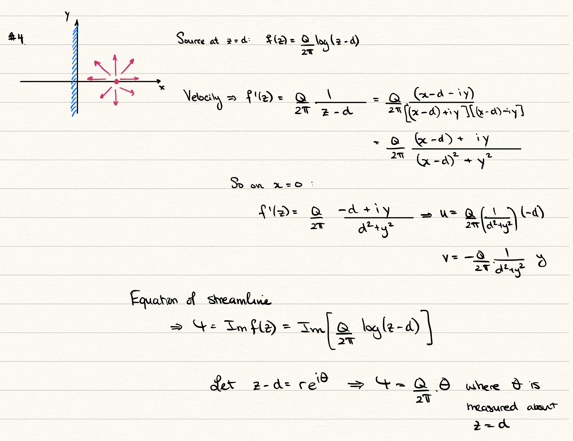
4.7.5. A source in a semi-infinite flow.

4.7.5.a

Solution.

4.7.5.b

Solution.

Since \(\psi = \frac{Q}{2\pi}\operatorname{Arg}(z^2 - d^2)\text{,}\) a streamline \(\psi = \textrm{constant}\) is a curve on which \(\operatorname{Arg}(z^2 - d^2) = \beta\) is constant. With \(z = x + \im y\text{,}\)

\begin{equation*} z^2 - d^2 = (x^2 - y^2 - d^2) + 2\im xy. \end{equation*}

Writing \(z^2 - d^2 = |z^2 - d^2|\e^{\im\beta}\text{,}\) the real and imaginary parts are \(|z^2 - d^2|\cos\beta\) and \(|z^2 - d^2|\sin\beta\text{.}\) Taking their ratio,

\begin{equation*} \frac{2xy}{x^2 - y^2 - d^2} = \tan\beta. \end{equation*}

4.7.5.c

Solution.

Multiplying out and writing \(k = \cot\beta\text{,}\) the streamlines are

\begin{equation*} x^2 - 2kxy - y^2 = d^2. \end{equation*}

This is a conic with \(A = 1\text{,}\) \(B = -2k\) and \(C = -1\text{,}\) so \(B^2 - 4AC = 4k^2 + 4 \gt 0\text{,}\) and each streamline is a hyperbola. Since \(A + C = 0\text{,}\) these are rectangular hyperbolae, and all of them pass through the two sources at \((\pm d, 0)\text{.}\) The limiting case \(\tan\beta = 0\) gives \(xy = 0\) away from the sources, i.e. the coordinate axes; in particular, the wall \(x = 0\) is a streamline, as required.

4.7.6. Two vortices and a dividing boundary.

Solution.

4.7.7. A line source in a flow; stagnation points.

Solution.

The potential is given by

\begin{equation*} f(z) = Uz + \frac{Q}{2\pi} [\log(z - a\im) + \log(z + a\im)] = Uz + \frac{Q}{2\pi} \log(z^2 + a^2). \end{equation*}

The complex velocity is then

\begin{equation*} f'(z) = U + \frac{Qz}{\pi(z^2 + a^2)}. \end{equation*}

A stagnation point requires \(f'(z) = 0\) and so we solve the resultant quadratic to obtain

\begin{equation*} z = \frac{-Q \pm \sqrt{Q^2 - (2a\pi U)^2}}{2\pi U}. \end{equation*}

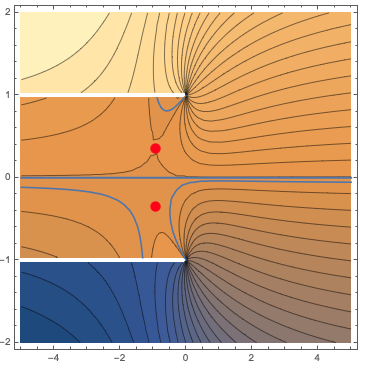
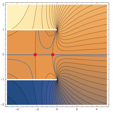
Setting \(\beta = Q/(2\pi a U)\text{,}\) there are two real roots if \(\beta > 1\text{.}\) Hence this is the case of two stagnation points along the axis. If \(\beta < 1\text{,}\) then there two complex conjugate points, and hence only one stagnation point in the flow field.

4.7.8. The exponential and sinusoidal conformal maps.

Solution.

For the exponential map, \(\zeta = \e^{\pi z/h}\text{,}\) we want to check the outputs of points A, B, C, D listed on the figure. These are as follows.

Table 4.22. Exponential map

\(z\)-plane	\(\zeta\)-plane
\(-\infty + \im h\)	\(0^-\)
\(\infty + \im h\)	\(-\infty\)
\(\infty\)	\(+\infty\)
\(-\infty\)	\(0^+\)

When thinking of the map, the most important step is to just verify that the line, \(z = t + \im h\text{,}\) is mapped to \(\zeta = -\e^{\pi t/h}\text{,}\) so the effect of shifting vertically by \(\im h\) is to negate the values as compared to evaluating on \(z = t\text{.}\) To verify the region the fluid is in, simply "walk" from ABCD in the \(z\)-plane, and remark on the orientation of the fluid relative to your journey (the fluid is on the right). The direction is preserved also in the \(\zeta\)-plane.

The potential that corresponds to a single source is found by using method of images in the \(\zeta\) plane and mapping backwards. It is

\begin{align*} F(\zeta) \amp= \frac{Q}{2\pi} \left[\log(\zeta - d) + \log(\zeta + \overline{d})\right], \\ f(z) \amp= \frac{Q}{2\pi} \left[\log(\e^{\pi z/h} - d) + \log(\e^{\pi z/h} + \overline{d})\right], \end{align*}

For the trigonometric map, \(\zeta = \sin(\pi z/2a)\text{,}\) the work is similar.

Table 4.23. Trigonometric map

\(z\)-plane	\(\zeta\)-plane
\(-a + \im \infty\)	\(-\infty\)
\(-a\)	\(-1\)
\(0\)	\(0\)
\(a\)	\(1\)
\(a + \im \infty\)	\(\infty\)

The potential that corresponds to a single source is found by using method of images in the \(\zeta\) plane and mapping backwards. It is

\begin{align*} F(\zeta) \amp= \frac{Q}{2\pi} \left[\log(\zeta - d) + \log(\zeta + \overline{d})\right], \\ f(z) \amp= \frac{Q}{2\pi} \left[\log(\sin(\pi z/2a) - d) + \log(\sin(\pi z/2a) + \overline{d})\right], \end{align*}

4.7.9. Elementary conformal maps.

Solution.

A conformal map is a mapping \(\zeta = g(z)\) where \(g\) is analytic and its derivative is nonzero in some region of the complex plane.

The map from the wedge to the upper half-plane is given in the notes near (4.5.1). It is \(\zeta = z^{\pi/\alpha}\text{.}\) The points where the mapping is not conformal are the critical points listed in the figure Figure 4.13. Point A at infinity is mapped directly to +infinity. The origin is mapped to the origin. And the point, B, found via \(z = r\e^{\im\alpha}\text{,}\) is sent to \(\zeta = -r^{\pi/\alpha}\) and then afterwards \(r \to \infty\text{.}\)

4.7.10. Flow past a flat plate.

4.7.10.a

Solution.

4.7.10.b

Solution.

4.7.10.c

Solution.

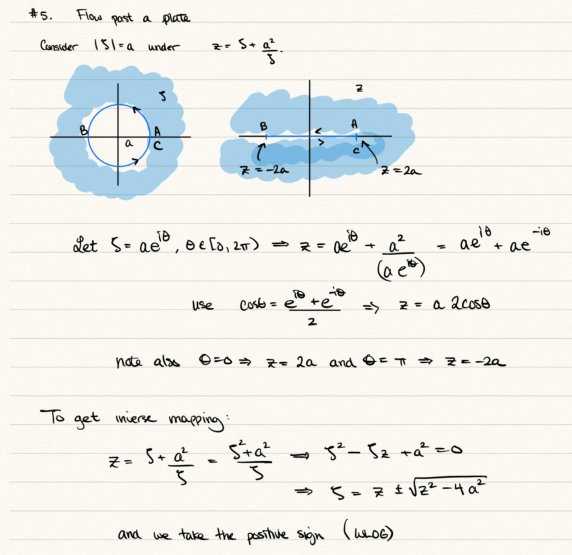
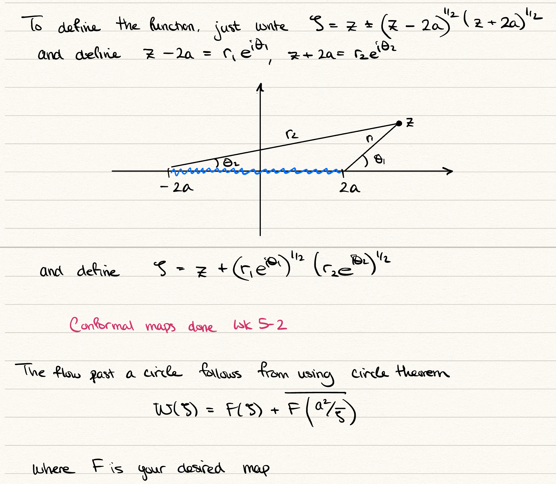
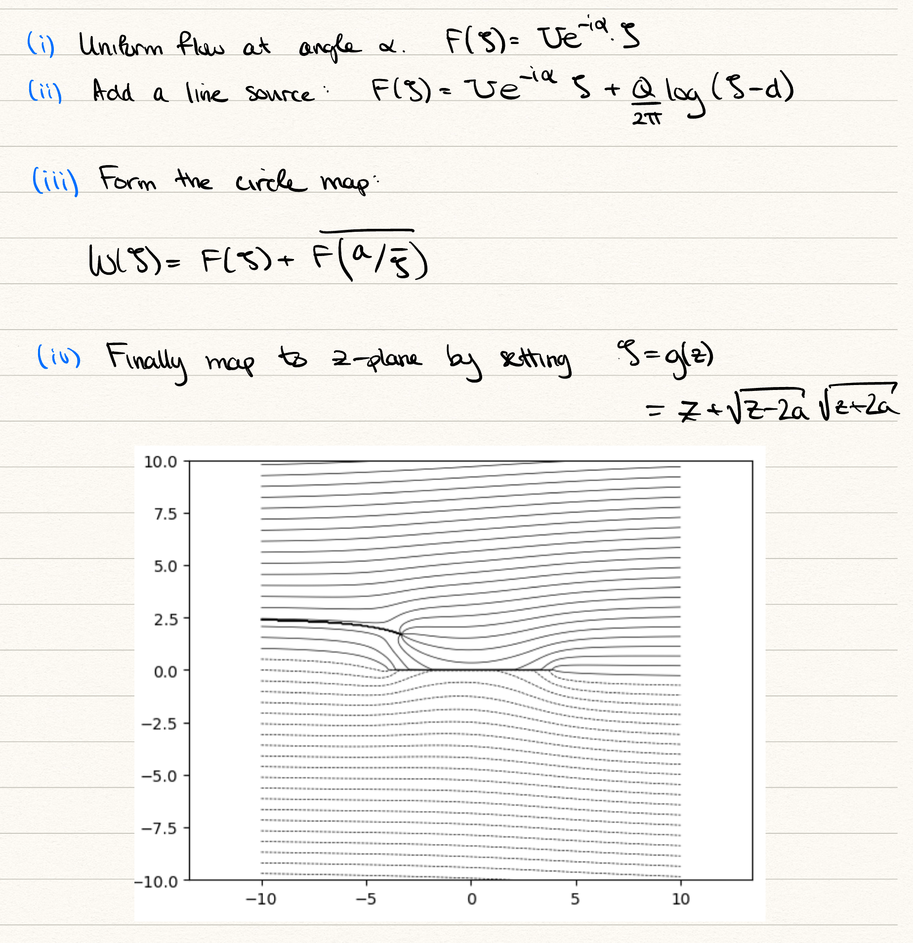
First, construct the complex potential \(F(\zeta)\) of uniform flow plus a source. Use the Circle Theorem (Theorem 4.6.1) to obtain the corresponding flow past a circular cylinder of radius \(a\text{.}\) Finally, use the map from part (b) to obtain the flow in the \(z\)-plane.

Prev Top Next