Section A.5 Viscous flows

Solutions Solutions

6.9 Practice Exercises

6.9.1. Reynolds number estimation.

6.9.1.a
Solution.
The kinematic viscosity of air at standard temperature and pressure is about \(1.5\times10^{-5}~\textrm{m}^2/\textrm{s}\text{.}\) The wingspan of a jumbo jet is about \(60~\textrm{m}\text{,}\) so the Reynolds number is approximately
\begin{equation*} \textrm{Re}=\frac{UL}{\nu} =\frac{150\times60}{1.5\times10^{-5}} =6\times10^8. \end{equation*}
6.9.1.b
Solution.
The kinematic viscosity of blood is about \(2.4\times10^{-6}~\textrm{m}^2/\textrm{s}\text{.}\) The diameter of the artery is about \(0.02~\textrm{m}\text{,}\) so the Reynolds number is approximately
\begin{equation*} \textrm{Re}=\frac{UL}{\nu} =\frac{0.3\times0.02}{2.4\times10^{-6}} =2500. \end{equation*}
Although this is above 2000, blood flow in arteries is typically laminar.
6.9.1.c
Solution.
The kinematic viscosity of honey is about \(0.007~\textrm{m}^2/\textrm{s}\text{.}\) The thickness of the layer is about \(0.005~\textrm{m}\text{,}\) so the Reynolds number is approximately
\begin{equation*} \textrm{Re}=\frac{UL}{\nu} =\frac{0.01\times0.005}{0.007} \approx0.007. \end{equation*}
6.9.1.d
Solution.
The kinematic viscosity of water at room temperature is about \(10^{-6}~\textrm{m}^2/\textrm{s}\text{.}\) The length of the tail is about \(10^{-3}~\textrm{m}\text{,}\) so the Reynolds number is approximately
\begin{equation*} \textrm{Re}=\frac{UL}{\nu} =\frac{100\times10^{-6}\times10^{-3}}{10^{-6}} =0.1. \end{equation*}

6.9.2. Nondimensionalisation.

6.9.2.a
Solution.
At the cylinder surface, we have the no-slip and no-penetration boundary conditions:
\begin{equation*} u=v=0. \end{equation*}
Far from the cylinder, the velocity approaches the uniform flow:
\begin{equation*} u\rightarrow U,\quad v\rightarrow0\quad\textrm{as }\sqrt{x^2+y^2}\rightarrow\infty. \end{equation*}
6.9.2.b
Solution.
We have:
\begin{equation*} \frac{U^2}{a}\left(\bu^*\cdot\nabla^*\right)\bu^* =-\frac{U^2}{a}\nabla^*p^* +\frac{\nu U}{a^2}\nabla^{*2}\bu^*,\quad \frac{U}{a}\nabla^*\cdot\bu^*=0, \end{equation*}
which simplify to
\begin{equation*} \mathrm{Re}\left(\bu^*\cdot\nabla^*\right)\bu^* =-\mathrm{Re}\nabla^*p^* +\nabla^{*2}\bu^*,\quad \nabla^*\cdot\bu^*=0, \end{equation*}
where
\begin{equation*} \mathrm{Re}=\frac{\rho Ua}{\mu} \end{equation*}
is the Reynolds number of the flow. The boundary conditions become:
\begin{equation*} u^*=v^*=0 \end{equation*}
at \(x^{*2}+y^{*2}=1\) and
\begin{equation*} u^*\rightarrow 1,\quad v^*\rightarrow0\quad\textrm{as }\sqrt{x^{*2}+y^{*2}}\rightarrow\infty. \end{equation*}

6.9.3. Falling ball viscometer.

6.9.3.a
Solution.
The dimensions of the terms are as follows:
\begin{equation*} [3\pi]=1,\quad [\mu]=ML^{-1}T^{-1},\quad [D]=L,\quad [u]=LT^{-1}, \end{equation*}
meaning that
\begin{equation*} \left[3\pi\mu Du\right]=1\times ML^{-1}T^{-1}\times L\times LT^{-1} =MLT^{-2}. \end{equation*}
Thus the expression \(3\pi\mu Du\) for the Stokes drag has the dimensions of force, as expected.
6.9.3.c
Solution.
Newton’s second law gives
\begin{equation*} m\frac{du}{dt}=mg-3\pi\mu Du. \end{equation*}
6.9.3.d
Solution.
We have
\begin{equation*} \frac{du}{dt}+\frac{3\pi\mu D}{m}u=g, \end{equation*}
for which the integrating factor is \(e^{\frac{3\pi\mu D}{m}t}\text{,}\) and
\begin{equation*} ue^{\frac{3\pi\mu D}{m}t}=\int ge^{\frac{3\pi\mu D}{m}t}dt =\frac{mg}{3\pi\mu D}e^{\frac{3\pi\mu D}{m}t}+c, \end{equation*}
where \(c\) is a constant of integration. Hence
\begin{equation*} u=\frac{mg}{3\pi\mu D}+ce^{-\frac{3\pi\mu D}{m}t} \end{equation*}
The initial condition is \(u=0\) at \(t=0\text{,}\) and, substituting this into the above equation, \(0=\frac{mg}{3\pi\mu D}+c\text{,}\) giving \(c=-\frac{mg}{3\pi\mu D}\text{.}\) Hence
\begin{equation*} u=\frac{mg}{3\pi\mu D}\left(1-e^{-\frac{3\pi\mu D}{m}t}\right). \end{equation*}
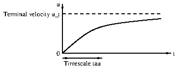
We substitute \(u_t=\frac{mg}{3\pi\mu D}\) and \(\tau=\frac{m}{3\pi\mu D}\text{.}\) With these substitutions we get
\begin{equation*} u=u_t\left(1-e^{-t/\tau}\right). \end{equation*}
The physical significance of these choices is that \(u_t\) is the terminal velocity of the sphere and \(\tau\) is the timescale over which the velocity of the sphere approaches the terminal velocity. Every \(\tau\) units of time, the velocity of the sphere becomes closer to the terminal velocity \(u_t\) by a factor \(e\approx2.7\text{.}\)
6.9.3.f
Solution.
Using the fact that the volume of a sphere is \(\pi D^3/6\text{,}\) where \(D\) is the diameter, we have \(m=\pi\rho_sD^3/6\text{,}\) where \(\rho_s=8,000\) kg/m\(^3\text{.}\) Thus
\begin{align*} u_t=&\frac{mg}{3\pi\mu D}=\frac{mg}{3\pi\mu D}=\frac{\rho_sgD^2}{18\mu}\\ =&\frac{8000\times9.81\times(4\times10^{-6})}{18\times1.2} =0.0146\,\textrm{m/s}=14.6\,\textrm{mm/s}. \end{align*}
The timescale \(\tau\) is given by
\begin{equation*} \tau=\frac{m}{3\pi\mu D}=\frac{\rho_sD^2}{18\mu} =\frac{8000\times4\times10^{-6}}{18\times1.2} =0.00148\,\textrm{s}. \end{equation*}
6.9.3.g
Solution.
The ball would attain its terminal velocity very quickly (in much less than a second), and since \(u_t\) is on order of centimetres per second, a container of about 10 cm deep would be suitable for measurement. In fact this idea is commonly used to measure the viscosity of fluids (since the viscosity can be calculated from the terminal velocity); this is called a falling ball viscometer.

6.9.4. Stress on a plate.

6.9.4.a
Solution.
We apply no-slip boundary conditions at the plate. Thus if \(y=kx\) then we must have \(u=0\) and \(v=0\text{.}\) Hence
\begin{equation*} 0=\alpha kx+Ax+B,\quad 0=-Akx+Dx+C, \end{equation*}
for all \(x\text{,}\) which implies that \(\alpha k+A=0\text{,}\) \(B=0\text{,}\) \(-Ak+D=0\) and \(C=0\text{.}\) Solving, we obtain
\begin{equation*} A=-\alpha k,\quad B=0,\quad D=-\alpha k^2,\quad C=0. \end{equation*}
Hence
\begin{equation*} u=\alpha\left(y-kx\right),\quad v=\alpha k\left(y-kx\right). \end{equation*}
6.9.4.b
Solution.
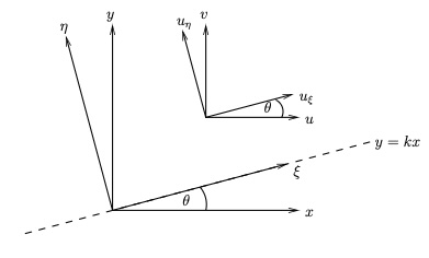
We perform the coordinate transform illustrated in FigureΒ 6.35 from the \((x,y)\)-plane to the \((\xi,\eta)\)-plane:
Figure 6.35. Sketch of plate.
We use
\begin{align*} \bu=&u\boldsymbol{i}+v\boldsymbol{j}\\ =&u\left(\cos\theta\hat{\boldsymbol{\xi}}-\sin\theta\hat{\boldsymbol{\eta}}\right) +v\left(\sin\theta\hat{\boldsymbol{\xi}}+\cos\theta\hat{\boldsymbol{\eta}}\right)\\ =&\left(u\cos\theta+v\sin\theta\right)\hat{\boldsymbol{\xi}} +\left(-u\sin\theta+v\cos\theta\right)\hat{\boldsymbol{\eta}}\\ =&\frac{\alpha(y-kx)+\alpha k^2(y-kx)}{\sqrt{1+k^2}}\hat{\boldsymbol{\xi}} +\frac{-\alpha k(y-kx)+\alpha k(y-kx)}{\sqrt{1+k^2}}\hat{\boldsymbol{\eta}}\\ =&\alpha\sqrt{1+k^2}(y-kx)\hat{\boldsymbol{\xi}}\\ =&\alpha\sqrt{1+k^2}\sqrt{1+k^2}\eta\hat{\boldsymbol{\xi}}\\ =&\alpha(1+k^2)\eta\hat{\boldsymbol{\xi}} \end{align*}
and so the velocity components are \(u_\xi=\alpha(1+k^2)\eta\) and \(u_\eta=0\text{.}\)
Thus the shear stress is given by
\begin{equation*} \mu\pd{u_\xi}{\eta}=\mu\alpha(1+k^2), \end{equation*}
and hence the drag force equals
\begin{equation*} \mu\alpha(1+k^2)LW. \end{equation*}
6.9.4.c
Solution.
We have the normal vector to the plate
\begin{equation*} \hat{\bn}=\frac1{\sqrt{1+k^2}}(-k,1,0). \end{equation*}
The rate-of-strain tensor is given by
\begin{equation*} \be=\left(\begin{matrix} -\alpha k&\frac12\alpha(1-k^2)&0\\ \frac12\alpha(1-k^2)&\alpha k&0\\ 0&0&0 \end{matrix}\right). \end{equation*}
Hence the stress tensor equals
\begin{equation*} \bsigma=-p\bI+2\mu\be =\left(\begin{matrix} -p-2\mu\alpha k&\mu\alpha(1-k^2)&0\\ \mu\alpha(1-k^2)&-p+2\mu\alpha k&0\\ 0&0&-p \end{matrix}\right). \end{equation*}
The stress on the surface is given by
\begin{align*} \tau=&\bsigma\hat{\bn}\\ =&\frac1{\sqrt{1+k^2}}\left(kp+2\mu\alpha k^2+\mu\alpha(1-k^2),-\mu k\alpha(1-k^2)-p+2\mu\alpha k,0\right)\\ =&\frac1{\sqrt{1+k^2}}\left(kp+\mu\alpha(1+k^2),-p+\mu k\alpha(1+k^2),0\right)\\ =&\frac1{\sqrt{1+k^2}}\left(p(k,-1,0)+\mu\alpha(1+k^2)(1,k,0)\right)\\ =&-p\hat{\bn}+\mu\alpha(1+k^2)\hat{\bt}, \end{align*}
where \(\hat{\bt}\) is the unit tangential vector to the plate in the \((x,y)\)-plane.
This is the pressure pushing into the plate (direction \(-\hat{\bn}\)) plus the drag \(\mu\alpha(1+k^2)\) along the plate. Hence, the total drag force is the drag times the area:
\begin{equation*} \mu\alpha(1+k^2) \end{equation*}
which agrees with the previous answer.

6.9.5. Stress on a surface due to the pressure.

6.9.5.a
Solution.
The force on \(x=x_0\) is pressure times area acting into the cube, which is \(\delta^2p|_{x_0}\bi\text{,}\) while the force on \(x=x_0+\delta\) equals \(-\delta^2p|_{x+\delta}\bi\text{.}\) Hence the contribution to the force from these two faces is
\begin{equation*} \delta^2p|_{x_0}\bi-\delta^2p|_{x+\delta}\bi \approx-\delta^3\pd{p}{x}\bi=-V\pd{p}{x}\bi. \end{equation*}
6.9.5.b
Solution.
The force on \(y=y_0\) is \(\delta^2p|_{y_0}\bj\) and that on \(y=y_0+\delta\) is \(-\delta^2p|_{y+\delta}\bj\text{.}\) This gives a contribution
\begin{equation*} \delta^2p|_{y_0}\bj-\delta^2p|_{y+\delta}\bj \approx-\delta^3\pd{p}{y}\bj=-V\pd{p}{y}\bj. \end{equation*}
Similarly, the force on \(z=z_0\) is \(\delta^2p|_{z_0}\bk\) and that on \(z=z_0+\delta\) is \(-\delta^2p|_{z+\delta}\bk\text{.}\) This gives a contribution
\begin{equation*} \delta^2p|_{z_0}\bk-\delta^2p|_{z+\delta}\bk \approx-\delta^3\pd{p}{z}\bk=-V\pd{p}{z}\bk. \end{equation*}
Hence the total force on the fluid in the cube due to the pressure of the surrounding fluid is given by
\begin{equation*} -V\pd{p}{x}\bi-V\pd{p}{y}\bj-V\pd{p}{z}\bk=-V\nabla p. \end{equation*}
6.9.5.c
Solution.
The unit normal to the face \(x=x_0\) is \(\hat{\bn}=-\bi\text{,}\) and hence the stress at a point in this face is
\begin{equation*} \tau=\bsigma\hat{\bn}=-p\bI(-\bi)=p\bi. \end{equation*}
Hence the force on this face equals \(\delta^2p_{x=x_0}\bi\text{.}\) Similarly, the unit normal to the face \(x=x_0+\delta\) is \(\hat{\bn}=\bi\text{,}\) and hence the stress at a point in this face is
\begin{equation*} \tau=\bsigma\hat{\bn}=-p\bI(\bi)=-p\bi. \end{equation*}
Hence the force on this face equals \(-\delta^2p_{x=x_0+\delta}\bi\text{.}\) Thus the contribution to the force from these two faces is
\begin{equation*} \delta^2p|_{x_0}\bi-\delta^2p|_{x+\delta}\bi \approx-\delta^3\pd{p}{x}\bi=-V\pd{p}{x}\bi. \end{equation*}
The contributions from the other faces can be calculated similarly, and the total force on the fluid in the cube due to the pressure of the surrounding fluid is given by
\begin{equation*} -V\pd{p}{x}\bi-V\pd{p}{y}\bj-V\pd{p}{z}\bk=-V\nabla p. \end{equation*}

6.9.6. Analysis of flow in a channel.

6.9.6.a
Solution.
The no-slip boundary conditions give
\begin{equation*} \bu(x,-h,z)=0,\quad \bu(x,h,z)=0 \end{equation*}
for all \(x\) and \(z\text{.}\)
6.9.6.b
Solution.
Since the plates are infinite in the \(x\) and \(z\) directions, and the pressure gradient is constant, there is no preferred location in these directions, and hence the velocity profile is independent of \(x\) and \(z\text{.}\) Furthermore, since there is no pressure gradient in the \(z\) direction, there is no driving force for flow in this direction, and hence the \(z\)-component of the velocity is zero (\(w=0\)).
6.9.6.c
Solution.
The continuity equation for an incompressible fluid is
\begin{equation*} \pd{u}{x}+\pd{v}{y}+\pd{w}{z}=0. \end{equation*}
Since the velocity is independent of \(x\) and \(z\text{,}\) the first and third terms are zero, and hence
\begin{equation*} \pd{v}{y}=0. \end{equation*}
Since the plates are rigid boundaries, there is no flow through them, and hence the no-penetration boundary conditions give
\begin{equation*} v(x,-h,z)=0,\quad v(x,h,z)=0 \end{equation*}
for all \(x\) and \(z\text{.}\) Since \(v\) is independent of \(y\) and zero at both \(y=-h\) and \(y=h\text{,}\) it follows that \(v=0\) for all \(y\text{.}\)
6.9.6.d
Solution.
At \(y=-h\text{,}\) we have
\begin{equation*} u(-h)=\frac{P}{2\mu}\left(h^2-(-h)^2\right) =\frac{P}{2\mu}(h^2-h^2)=0, \end{equation*}
and at \(y=h\text{,}\) we have
\begin{equation*} u(h)=\frac{P}{2\mu}\left(h^2-h^2\right) =\frac{P}{2\mu}(h^2-h^2)=0. \end{equation*}
Hence the profile satisfies the boundary conditions.
6.9.6.e
Solution.
A larger pressure gradient \(P\) means a larger driving force for the flow, and hence a larger velocity. A larger viscosity \(\mu\) means a larger resistance to the flow, and hence a smaller velocity. Therefore, it is to be expected that the velocity profile increases as \(P\) increases and decreases as \(\mu\) increases.
6.9.6.f
Solution.
The pressure at a general point is given by
\begin{equation*} p=p_0-Px. \end{equation*}
At \(y=-h\text{,}\) the normal stress is given by the pressure, pointing into the plate:
\begin{equation*} \tau_y=-p=-p_0+Px. \end{equation*}
(note the negative sign as "into the plate" is in the \(-y\)-direction). The \(x\)-component of the shear stress at \(y=-h\) is given by
\begin{equation*} \tau_x=\mu\pd{u}{y}=\mu\pd{}{y}\left[\frac{P}{2\mu}(h^2-y^2)\right] =\mu\left(-\frac{P}{\mu}y\right)=Ph \end{equation*}
(note that this is positive since the fluid is pushing the plate in the positive \(x\)-direction). The \(z\)-component of the shear stress at \(y=-h\) is zero since \(w=0\text{.}\) Hence
\begin{equation*} \tau=(Ph,-p_0+Px,0). \end{equation*}
At \(y=h\text{,}\) the normal stress is given by the pressure, pointing into the plate:
\begin{equation*} \tau_y=p_0-Px \end{equation*}
(note the sign change compared to the previous part as "into the plate" is in the \(+y\)-direction). The \(x\)-component of the shear stress at \(y=h\) is given by
\begin{equation*} \tau_x=-\mu\pd{u}{y}=-\mu\pd{}{y}\left[\frac{P}{2\mu}(h^2-y^2)\right] =-\mu\left(-\frac{P}{\mu}y\right)=Ph. \end{equation*}
Note that the formula used has a negative sign as "into the fluid" is in the \(-y\)-direction. The overall sign is positive since the fluid is pushing the plate in the positive \(x\)-direction. (It is good to check signs after this kind of calculation by checking the direction of the force.) The \(z\)-component of the shear stress at \(y=h\) is zero since \(w=0\text{.}\) Hence
\begin{equation*} \tau=(Ph,p_0-Px,0). \end{equation*}
6.9.6.g
Solution.
The normal stresses on the two plates are equal in magnitude but opposite in direction, as expected since the pressure acts equally on both plates, but "into the plates" is a different direction.
The shear stresses on the two plates are equal in magnitude and direction, indicating that the fluid is exerting the same tangential force on both plates in the direction of the flow. This is also expected since the plane \(y=0\) is a plane of symmetry.

6.9.7. Force on a blob of fluid.

6.9.7.a
Solution.
The \(i\)th component of
\begin{equation*} \hat{\bn}\times\left(\nabla\times\bu\right) =\nabla(\hat{\bn}\cdot\bu)-(\hat{\bn}\cdot\nabla)\bu, \end{equation*}
is
\begin{align*} \left[\hat{\bn}\times(\nabla\times\bu)\right]_i &=\sum_{j=1}^3n_j\pd{u_j}{x_i}-(\hat{\bn}\cdot\nabla)u_i\\ &=\sum_{j=1}^3n_j\pd{u_j}{x_i}-\sum_{j=1}^3n_j\pd{u_i}{x_j}. \end{align*}
Hence, the \(i\)th component of the target expression is
\begin{align*} &\left\{-p\bn+\mu\left[2(\hat{\bn}\cdot\nabla)\bu +\hat{\bn}\times(\nabla\times\bu)\right]\right\}_i\\ &=-pn_i+\mu\left[2\sum_{j=1}^3n_j\pd{u_i}{x_j} +\sum_{j=1}^3n_j\pd{u_j}{x_i}-\sum_{j=1}^3n_j\pd{u_i}{x_j}\right]\\ &=-pn_i+\mu\left[\sum_{j=1}^3n_j\pd{u_i}{x_j} +\sum_{j=1}^3n_j\pd{u_j}{x_i}\right]\\ &=\sum_{j=1}^3\left[-p\delta_{ij}+\mu\left(\pd{u_i}{x_j} +\pd{u_j}{x_i}\right)\right]n_j\\ &=\sum_{j=1}^3\sigma_{ij}n_j\\ &=\btau_i, \end{align*}
as required.
6.9.7.b
Solution.
We have
\begin{align*} \bf=&\iint_S\btau\de S\\ =&\iint_S\left\{-p\hat{\bn}+\mu\left[2(\hat{\bn}\cdot\nabla)\bu +\hat{\bn}\times(\nabla\times\bu)\right]\right\}\de S. \end{align*}
We now make use of the vector calculus identities given in the hint. The first term becoems
\begin{equation*} \iint_S-p\hat{\bn}\de S=\iiint_V-\nabla p\de V, \end{equation*}
the second term becomes
\begin{equation*} \iint_S2\mu(\hat{\bn}\cdot\nabla)\bu\de S =\iiint_V2\mu\nabla^2\bu\de V, \end{equation*}
and for the third term,
\begin{align*} \iint_S\mu\hat{\bn}\times(\nabla\times\bu)\de S =&-\iint_S\mu(\nabla\times\bu)\times\hat{\bn}\de S\\ =&\iiint_V\mu\nabla\times(\nabla\times\bu)\de V,\\ =&\iiint_V\mu\nabla(\nabla\cdot\bu)-\mu\nabla^2\bu\de V. \end{align*}
Hence, since the fluid is incompressible and \(\nabla\cdot\bu=0\text{,}\) the third term becomes
\begin{equation*} \\\int_V-\mu\nabla^2\bu\de V. \end{equation*}
Combining these three results gives
\begin{align*} \bF=&\iiint_V\left(-\nabla p+2\mu\nabla^2\bu-\mu\nabla^2\bu\right)\de V\\ =&\iiint_V\left(-\nabla p+\mu\nabla^2\bu\right)\de V, \end{align*}
as required.
6.9.7.c
Solution.
If the blob is small, then the integrand in the expression for the force varies little over the volume of the blob, and so
\begin{equation*} \bF\approx\left(-\nabla p+\mu\nabla^2\bu\right)V, \end{equation*}
where \(V\) is the volume of the blob. Hence the force per unit volume is given by
\begin{equation*} \frac{\bF}{V}=-\nabla p+\mu\nabla^2\bu, \end{equation*}
as required.

6.9.8. General deformation of a fluid element.

6.9.8.a
Solution.
The velocity at point \(Q\) can be expressed as a Taylor series expansion about point \(P\text{:}\)
\begin{equation*} \bu_Q=\bu_P+\left(\bs\cdot\nabla\right)\bu +\frac{1}{2!}\left(\bs\cdot\nabla\right)^2\bu +\frac{1}{3!}\left(\bs\cdot\nabla\right)^3\bu+\cdots. \end{equation*}
Since \(Q\) is a nearby point to \(P\text{,}\) the higher order terms in \(\bs\) are negligible, and hence we have
\begin{equation*} \bu_Q=\bu_P+(\bs\cdot\nabla)\bu, \end{equation*}
as required.
6.9.8.b
Solution.
We have that the \(k\)th component of the final term of the target expression is
\begin{align*} &\left\{\frac12\nabla_s(\sum_{i=1}^3\sum_{j=1}^3e_{ij}s_is_j)\right\}_k\\ =&\frac12\pd{}{s_k}(\sum_{i=1}^3\sum_{j=1}^3e_{ij}s_is_j)\\ =&\frac12(\sum_{i=1}^3e_{ik}s_i+\sum_{j=1}^3e_{kj}s_j)\\ =&\frac12\sum_{i=1}^3(e_{ik}s_i+e_{ki}s_i)\\ =&\sum_{i=1}^3e_{ik}s_i, \end{align*}
where the final equality uses the fact that the rate-of-strain tensor is symmetric \(e_{ij}=e_{ji}\text{.}\) Substituting for \(e_{ik}\) gives
\begin{align*} &\sum_{i=1}^3e_{ik}s_i\\ =&\frac12\sum_{i=1}^3\left(\pd{u_i}{x_k}+\pd{u_k}{x_i}\right)s_i. \end{align*}
Using the given vector identity, the \(k\)th component of the second term of the target expression is
\begin{align*} &\left\{\frac12(\nabla_x\times\bu)\times\bs\right\}_k\\ =&\frac12\left\{\bs\cdot\nabla_x\bu-\nabla_x(\bs\cdot\bu)\right\}_k\\ =&\frac12\left\{\sum_{i=1}^3s_i\pd{u_k}{x_i} -\sum_{i=1}^3s_i\pd{u_i}{x_k}\right\}\\ =&\frac12\sum_{i=1}^3\left(\pd{u_k}{x_i}-\pd{u_i}{x_k}\right)s_i. \end{align*}
Hence the \(k\)th component of the sum of the second and the third terms of the target expression is
\begin{align*} &\frac12(\nabla_x\times\bu)\times\bs +\frac12\nabla_s(\sum_{i=1}^3\sum_{j=1}^3e_{ij}s_is_j)\\ =&\frac12\sum_{i=1}^3\left(\pd{u_k}{x_i}-\pd{u_i}{x_k}\right)s_i +\frac12\sum_{i=1}^3\left(\pd{u_i}{x_k}+\pd{u_k}{x_i}\right)s_i\\ =&\sum_{i=1}^3\pd{u_k}{x_i}s_i, \end{align*}
which is the \(k\)th component of \((\bs\cdot\nabla)\bu\text{,}\) thus proving the result.
6.9.8.c
Solution.
  • The first term \(\bu_P\) represents translation since it is the velocity at point \(P\text{.}\)
  • The second term \(\frac12(\nabla_x\times\bu)\times\bs\) represents rotation since, setting \(\bOmega=\nabla_x\times\bu/2=\bomega/2\text{,}\) this term is of the form \(\bOmega\times\bs\text{,}\) which is purely rotational motion about point \(P\) (see ExerciseΒ 6.10.2). Note also that this shows that the vorticity \(\bomega\) is twice the local angular velocity of the fluid element, since \(\bOmega=\bomega/2\text{.}\) This makes precise the statement in DefinitionΒ 3.5.2 that the vorticity measures the local rotation of the flow.
  • The third term \(\frac12\nabla_s(\sum_{i=1}^3\sum_{j=1}^3e_{ij}s_is_j)\) represents pure strain since it depends on the rate-of-strain tensor \(e_{ij}\text{,}\) which describes how the fluid element is deformed without rotation.

6.9.9. Decomposition of a shear flow.

6.9.9.a
Solution.
(ii) The vorticity
\begin{equation*} \bomega=(0,0,-\beta), \end{equation*}
and therefore the rotational component is
\begin{equation*} \frac12\bomega\times\bs =\frac12\beta(s_y,-s_x,0), \end{equation*}
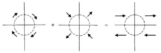
which is clockwise rotation with angular velocity \(\beta/2\text{,}\) see left sketch in FigureΒ 6.36.
(iii) We have the rate-of-strain tensor
\begin{equation*} \be=\left(\begin{matrix} 0&\beta/2&0\\ \beta/2&0&0\\ 0&0&0 \end{matrix}\right). \end{equation*}
Hence
\begin{equation*} \frac12\nabla_s\left(\sum_{j=1}^3\sum_{i=1}^3e_{ij}s_is_j\right) =\frac{\beta}2\nabla_s\left(s_1s_2\right) =\frac{\beta}2\left(s_y,s_x,0\right) \end{equation*}
(note that we are interchanging between \(s=(s_1,s_2,s_3)\) and \((s_x,s_y,s_z)\)). The eigenvalues \(\lambda\) of \(\be\) satisfy
\begin{equation*} -\lambda^3+\frac14\beta^2\lambda=0, \end{equation*}
which has solutions \(\lambda=0,\pm\beta/2\text{.}\) The associated eigenvectors are
\begin{equation*} \hat{\mathbf{k}}, \quad\left(\frac1{\sqrt{2}},\frac1{\sqrt{2}},0\right), \quad\left(-\frac1{\sqrt{2}},\frac1{\sqrt{2}},0\right). \end{equation*}
This corresponds to expansion along the line \(x=y\) and contraction along \(x=-y\text{,}\) see middle sketch in FigureΒ 6.36.
The solution is illustrated in FigureΒ 6.36.
Figure 6.36. Sketches showing the decomposition of the flow into rotation (left) and pure straining flow (middle), with the total flow shown on the right.

6.9.10. Derivation of the Cauchy equation.

6.9.10.a
Solution.
We consider a volume \(V\) with surface \(S\) consisting of a small cube of side length \(\delta\text{,}\) as shown in FigureΒ 6.18. We apply the Reynolds Transport Theorem to the fluid in the cube:
\begin{equation*} \dd{}{t} \iiint_{V(t)} f \, \de{x} \, \de{y} \, \de{z} = \iiint_{V(t)} \left[ \pd{f}{t} + \nabla \cdot (f\bu)\right] \, \de{x} \, \de{y} \, \de{z}, \end{equation*}
where \(f\) is any function, a vector or a scalar.
Setting \(\bf=\rho\bu\) equal to the momentum per unit volume in the fluid, the integral equals the momentum of the fluid in the cube, and the time derivative is the rate of change of momentum, which is the total force acting on the fluid in the cube.
The total force equals the sum of the surface forces and body forces. The body force equals the force of gravity: \(\rho V\bg\text{.}\) The surface forces are an integral:
\begin{equation*} \iint_S\btau\,\de S=\iint_S\bsigma\bn\,\de S; \end{equation*}
and we sum the contributions over the six faces in pairs:
  • Front and back faces: The contribution on the back face (\(\bn=-\bi\)) is
    \begin{equation*} -\delta^2\left.\left(\begin{array}{c} \sigma_{11}\\\sigma_{12}\\\sigma_{13} \end{array}\right)\right|_{x=x_0} \end{equation*}
    and on the front face (\(\bn=\bi\)), it is
    \begin{equation*} \delta^2\left.\left(\begin{array}{c} \sigma_{11}\\\sigma_{12}\\\sigma_{13} \end{array}\right)\right|_{x=x_0+\delta}. \end{equation*}
    The sum of these is
    \begin{equation*} \delta^2\left.\left(\begin{array}{c} \sigma_{11}\\\sigma_{12}\\\sigma_{13} \end{array}\right)\right|_{x=x_0+\delta} -\delta^2\left.\left(\begin{array}{c} \sigma_{11}\\\sigma_{12}\\\sigma_{13} \end{array}\right)\right|_{x=x_0} =\delta^3\pd{}{x}\left(\begin{array}{c} \sigma_{11}\\\sigma_{12}\\\sigma_{13} \end{array}\right). \end{equation*}
  • Left and right faces: In a similar way, the contribution is
    \begin{equation*} \delta^3\pd{}{y}\left(\begin{array}{c} \sigma_{21}\\\sigma_{22}\\\sigma_{23} \end{array}\right). \end{equation*}
  • Bottom and top faces: The contribution is
    \begin{equation*} \delta^3\pd{}{z}\left(\begin{array}{c} \sigma_{31}\\\sigma_{32}\\\sigma_{33} \end{array}\right). \end{equation*}
Hence, the surface force is given by
\begin{equation*} \delta^3\pd{}{x}\left(\begin{array}{c} \sigma_{11}\\\sigma_{12}\\\sigma_{13} \end{array}\right) +\delta^3\pd{}{y}\left(\begin{array}{c} \sigma_{21}\\\sigma_{22}\\\sigma_{23} \end{array}\right) +\delta^3\pd{}{z}\left(\begin{array}{c} \sigma_{31}\\\sigma_{32}\\\sigma_{33} \end{array}\right) =\delta^3\nabla\cdot\bsigma, \end{equation*}
Hence
\begin{equation*} \rho V\bg+\delta^3\nabla\cdot\bsigma =\iiint_{V(t)} \left[\pd{(\rho\bu)}{t} + \nabla \cdot (\rho\bu\bu)\right]\,\de{x}\,\de{y}\,\de{z}, \end{equation*}
Since the cube is small, the right-hand side is approximately the volume \(V\) times the integrand evaluated at a point in \(V\text{.}\) Dividing by \(V=\delta^3\) gives
\begin{equation*} \rho\bg+\nabla\cdot\bsigma =\pd{(\rho\bu)}{t} + \nabla \cdot ((\rho\bu)\bu). \end{equation*}
Since \(\rho\) is constant,
\begin{equation*} \rho\bg+\nabla\cdot\bsigma =\rho\pd{\bu}{t} + \rho\bu\cdot\nabla\bu+\rho(\nabla\cdot\bu)\bu. \end{equation*}
Since the fluid is incompressible, we have \(\nabla\cdot\bu=0\text{,}\) and, rearranging, we obtain the Cauchy equation:
\begin{equation*} \rho\left(\pd{\bu}{t} + \bu\cdot\nabla\bu\right) =\nabla\cdot\bsigma+\rho\bg \end{equation*}
6.9.11. Limits of low and high Reynolds number.

6.9.11.a
Solution.
We have
\begin{equation*} \rho\pd{\bu}{t}+\rho\bu\cdot\nabla\bu=-\nabla p+\mu\nabla^2\bu+\rho{\bg},\quad \nabla\cdot\bu=0, \end{equation*}
which, after nondimensionalising, become
\begin{equation*} \frac{\rho U}{T}\pd{\bu^*}{t^*}+\frac{\rho U^2}{L}\bu^*\cdot\nabla^*\bu^* =-\frac{P}{L}\nabla^* p^*+\frac{\mu U}{L^2}\nabla^{*2}\bu^*+\rho g\hat{\bg},\quad \frac{U}{L}\nabla^*\cdot\bu^*=0. \end{equation*}
6.9.11.b
Solution.
We set the coefficients of the two inertial terms equal:
\begin{equation*} \frac{\rho U}{T}=\frac{\rho U^2}{L} \quad\Rightarrow\quad T=\frac{L}{U}. \end{equation*}
Multiplying the Navier–Stokes equation by \(L^2/(\mu U)\text{,}\) we get
\begin{equation*} \mathrm{Re}\DD{\bu^*}{t^*} =-\frac{LP}{\mu U}\nabla^* p^*+\nabla^{*2}\bu^*+\frac{\rho L^2g}{\mu U}\hat{\bg}. \end{equation*}
The coefficient multiplying the inertial terms is the Reynolds number \(\mathrm{Re}\text{.}\)
6.9.11.c
Solution.
In this case, the inertial terms are small compared to the viscous terms, so we can neglect them. The gravitational acceleration term has order of magnitude \(\rho L^2g/(\mu U)\text{.}\) We need to consider the cases in which this is large, order one or small:
  • If \(\rho L^2g/(\mu U)\gg1\text{,}\) the pressre have a predominantly hydrostatic pressure profile, with the fluid dynamical problem being a small perturbation to the background static problem. Thus the pressure gradient balances this term:
    \begin{equation*} \frac{LP}{\mu U}=\frac{\rho L^2g}{\mu U} \quad\Rightarrow\quad P=\rho Lg, \end{equation*}
    and, to leading order, the Navier–Stokes equation becomes
    \begin{equation*} 0=-\nabla^* p^*+\hat{\bg}. \end{equation*}
    Once we have solved this problem, we could in principle solve a secondary problem to find the fluid flow. Thus the dimensional problem is
    \begin{equation*} 0=-\nabla p+\rho\bg. \end{equation*}
  • If \(\rho L^2g/(\mu U)\) is of order 1, the gravitational acceleration term balances the leading-order terms in the equation, and we set
    \begin{equation*} \frac{LP}{\mu U}=1\quad\Rightarrow\quad P=\frac{\mu U}{L}. \end{equation*}
    We obtain the leading-order system
    \begin{equation*} 0=-\nabla^* p^*+\nabla^{*2}\bu^*+\frac{\rho L^2g}{\mu U}\hat{\bg}, \end{equation*}
    and redimensionalising, we get
    \begin{equation*} 0=-\nabla p+\mu\nabla^2\bu, \end{equation*}
    and the continuity equation is retained in full:
    \begin{equation*} \nabla\cdot\bu=0. \end{equation*}
  • If \(\rho L^2g/(\mu U)\ll1\text{,}\) the gravitational acceleration term is small compared to the leading-order terms in the equation, and we set
    \begin{equation*} \frac{LP}{\mu U}=1\quad\Rightarrow\quad P=\frac{\mu U}{L}. \end{equation*}
    We obtain the leading-order system
    \begin{equation*} 0=-\nabla^* p^*+\nabla^{*2}\bu^*, \end{equation*}
    and redimensionalising, we get
    \begin{equation*} 0=-\nabla p+\mu\nabla^2\bu, \end{equation*}
    and the continuity equation is retained in full:
    \begin{equation*} \nabla\cdot\bu=0. \end{equation*}
6.9.11.d
Solution.
In this case, the viscous terms are small compared to the inertial terms, so we can neglect them. Dividing the Navier–Stokes equation by \(\mathrm{Re}\text{,}\)
\begin{equation*} \DD{\bu^*}{t^*} =-\frac{P}{\rho U^2}\nabla^* p^*+\frac{Lg}{U^2}\hat{\bg}. \end{equation*}
The gravitational acceleration term now has order of magnitude \(Lg/U^2\text{.}\) We need to consider the cases in which this is large, order one or small:
  • If \(Lg/U^2\gg1\text{,}\) the pressre have a predominantly hydrostatic pressure profile, with the fluid dynamical problem being a small perturbation to the background static problem. Thus the pressure gradient balances this term:
    \begin{equation*} \frac{P}{\rho U^2}=\frac{Lg}{U^2} \quad\Rightarrow\quad P=\rho Lg, \end{equation*}
    and, to leading order, the Navier–Stokes equation becomes
    \begin{equation*} 0=-\nabla^* p^*+\hat{\bg}. \end{equation*}
    As in the low-Reynolds-number cases, once we have solved this problem, we could in principle solve a secondary problem to find the fluid flow. Thus the dimensional problem is
    \begin{equation*} 0=-\nabla p+\rho\bg. \end{equation*}
  • If \(Lg/U^2\) is of order 1, the gravitational acceleration term balances the leading-order terms in the equation, and we set
    \begin{equation*} \frac{P}{\rho U^2}=1\quad\Rightarrow\quad P=\rho U^2. \end{equation*}
    We obtain the leading-order system
    \begin{equation*} \DD{u^*}{t^*}=-\nabla^* p^*+\frac{Lg}{U^2}\hat{\bg}, \end{equation*}
    and redimensionalising, we get
    \begin{equation*} \rho\DD{u}{t}=-\nabla p+\rho\bg, \end{equation*}
    and the continuity equation is retained in full:
    \begin{equation*} \nabla\cdot\bu=0. \end{equation*}
  • If \(Lg/U^2\ll1\text{,}\) the gravitational acceleration term is small compared to the leading-order terms in the equation, and we set
    \begin{equation*} \frac{P}{\rho U^2}=1\quad\Rightarrow\quad P=\rho U^2. \end{equation*}
    We obtain the leading-order system
    \begin{equation*} \DD{u^*}{t^*}=-\nabla^* p^*, \end{equation*}
    and redimensionalising, we get
    \begin{equation*} \rho\DD{u}{t}=-\nabla p, \end{equation*}
    and the continuity equation is retained in full:
    \begin{equation*} \nabla\cdot\bu=0. \end{equation*}

6.9.12. Hagen–Poiseuille flow.

6.9.12.a
Solution.
We have that the volumetric flux along the pipe equals (\(A\) is a circular cross-section \(z=\mathrm{constant}\) of the pipe)
\begin{align*} Q=&\iint_Aw\,\de A\\ =&\int_0^{2\pi}\int_0^a\frac{G}{4\mu}\left(a^2-r^2\right)r\,\de r\,\de \theta\\ =&2\pi\frac{G}{4\mu}\int_0^a\left(a^2r-r^3\right)\,\de r\\ =&\frac{\pi G}{2\mu}\left[\frac{a^2r^2}{2}-\frac{r^4}{4}\right]_0^a\\ =&\frac{\pi G}{2\mu}\left(\frac{a^4}{2}-\frac{a^4}{4}\right)\\ =&\frac{\pi Ga^4}{8\mu}, \end{align*}
where \(G=\Delta p/L\) is the pressure gradient. Rearranging,
\begin{equation*} \Delta p=\frac{8\mu LQ}{\pi a^4}, \end{equation*}
as expected.

6.9.13. Flow outside a cylinder.

6.9.13.a
Solution.
Axisymmetry implies \(u_\theta=0\) and two-dimensional flow implies \(u_z=0\text{.}\) With these assumptions, the continuity equation becomes
\begin{equation*} \frac1r\pd{}{r}\left(ru_r\right)=0. \end{equation*}
Multiplying by \(r\) and integrating,
\begin{equation*} ru_r=A\quad\Rightarrow\quad u_r=\frac{A}{r}, \end{equation*}
where \(A\) is constant. The boundary condition on \(r=a\) reads \(u_r=-U\text{,}\) and hence
\begin{equation*} -U=\frac{A}{a}\quad\Rightarrow\quad A=-aU. \end{equation*}
Substituting this in,
\begin{equation*} u_r=\frac{-aU}{r}. \end{equation*}
6.9.13.b
Solution.
We substitute the assumptions into the Navier–Stokes equations, which state that all \(t\text{,}\) \(\theta\) and \(z\) derivatives are zero and \(u_\theta=u_z=0\text{.}\) The equations become:
\begin{align*} \rho u_r\pd{u_r}{r} =&-\pd{p}{r} +\mu\left(\nabla^2u_r-\frac{u_r}{r^2}\right),\\ 0=&0,\\ 0=&0, \end{align*}
and
\begin{equation*} \nabla^2u_r =\frac1r\pd{}{r}\left(r\pd{u_r}{r}\right) =\pd{^2u_r}{r^2}+\frac1r\pd{u_r}{r}. \end{equation*}
Hence, the only non-trivial equation is the \(r\)-component, which reduces to
\begin{equation*} \rho u_r\pd{u_r}{r} =-\pd{p}{r} +\mu\left(\pd{^2u_r}{r^2}+\frac1r\pd{u_r}{r}-\frac{u_r}{r^2}\right). \end{equation*}
Substituting the expression for \(u_r\text{,}\)
\begin{equation*} \rho \left(-\frac{aU}{r}\right)\left(\frac{aU}{r^2}\right) =-\pd{p}{r} +\mu\left(-\frac{2aU}{r^3}+\frac{aU}{r^3}+\frac{aU}{r^3}\right), \end{equation*}
which simplifies to
\begin{equation*} \pd{p}{r}=\frac{\rho a^2U^2}{r^3}, \end{equation*}
as required.
6.9.13.c
Solution.
We solve the equation, applying the boundary condition as \(r\rightarrow\infty\) to find that
\begin{equation*} \pd{p}{r}=p_0-\frac{\rho a^2U^2}{2r^2}. \end{equation*}

6.9.14. Oscillating flow in a pipe.

6.9.14.a
Solution.
We assume that the flow is axisymmetric and fully developed. The continuity equation reduces to
\begin{equation*} \frac1r\pd{}{r}\left(ru_r\right)=0, \end{equation*}
which implies that
\begin{equation*} u_r=\frac{A}{r} \end{equation*}
where \(A\) is independent of \(r\text{.}\) Regularity at \(r=0\) implies that \(A=0\text{,}\) and therefore \(u_r=0\) everywhere.
6.9.14.b
Solution.
With the assumptions, the Navier–Stokes equations reduce to
\begin{align*} 0=&-\pd{p}{r},\\ 0=&0,\\ \rho\im\omega Ue^{\im\omega t}+\mathrm{c.c.} =G_0\cos\omega t+\frac{\mu}{r}\dd{}{r}\left(rU'\right)e^{\im\omega t}+\mathrm{c.c.}. \end{align*}
There is thus one non-trivial component, and, taking the part proportional to \(e^{\im\omega t}\text{,}\) we have
\begin{equation*} \rho\im\omega U=\frac12G_0+\frac{\mu}{r}\dd{}{r}\left(rU'\right), \end{equation*}
which, dividing by \(\mu\text{,}\) is equivalent to
\begin{equation*} \frac{\im\rho\omega}{\mu} U=\frac{G_0}{2\mu}+U''+\frac1rU'. \end{equation*}
Rearranging gives the result.
6.9.14.c
Solution.
With this substitution, we have
\begin{equation*} \dd{}{r}=e^{-\im\pi/4}\alpha\dd{}{s}, \end{equation*}
and hence
\begin{equation*} -\im\alpha^2\dd{^2U}{s^2}-\im\alpha^2\frac1s\dd{U}{s} -\im\alpha^2U=-\frac{G_0}{2\mu}, \end{equation*}
giving
\begin{equation*} \dd{^2U}{s^2}+\frac1s\dd{U}{s}+U=-\frac{\im G_0}{2\rho\omega}. \end{equation*}
6.9.14.d
Solution.
For simplicity, seek a constant solution, and we find
\begin{equation*} U_{PI}=-\frac{\im G_0}{2\rho\omega}. \end{equation*}

6.9.15. Solving the Navier–Stokes equations in spherical polar coordinates.

6.9.15.a
Solution.
We assume the flow and pressure fields are steady and spherically symmetric. Thus we neglect all \(t\text{,}\) \(\theta\) and \(\phi\) derivatives, and set \(u_\theta=u_\phi=0\text{.}\) The continuity equation reduces to
\begin{equation*} \frac1{r^2}\pd{(r^2u_r)}{r}=0, \end{equation*}
which implies that
\begin{equation*} u_r=\frac{A}{r^2} \end{equation*}
where \(A\) is independent of \(r\text{.}\) The Navier–Stokes equations reduce to
\begin{align*} \rho u_r\pd{u_r}{r}=&-\pd{p}{r}+\mu\left(\frac1{r^2}\pd{}{r}\left(r^2\pd{u_r}{r}\right)-\frac{2u_r}{r^2}\right),\\ 0=&0,\\ 0=&0, \end{align*}
Substituting the expression for \(u_r\) into the \(r\)-component gives
\begin{equation*} -\frac{\rho A^2}{r^5}=-\pd{p}{r}+\mu\left(-\frac{2A}{r^4}+\frac{2A}{r^4}\right), \end{equation*}
which simplifies to
\begin{equation*} \pd{p}{r}=\frac{\rho A^2}{r^5}. \end{equation*}
Integrating and applying the boundary condition as \(r\rightarrow\infty\) gives
\begin{equation*} p=p_0-\frac{\rho A^2}{4r^4}. \end{equation*}
Applying the boundary condition at \(r=a\) gives
\begin{equation*} p_1=p_0-\frac{\rho A^2}{4a^4}\quad\Rightarrow\quad A=a^2\sqrt{\frac{4(p_0-p_1)}{\rho}}, \end{equation*}
and hence the velocity and pressure fields are
\begin{align*} u_r=&\frac{a^2}{r^2}\sqrt{\frac{4(p_0-p_1)}{\rho}},\\ p=&p_0-\frac{\rho a^4(p_0-p_1)}{r^4}. \end{align*}

6.10 Problems set 7 to hand in

6.10.1. Analysis of flow in a pipe.

6.10.1.a
Solution.
The no-slip boundary conditions give
\begin{equation*} \left.\bu\right|_{r=a}=0. \end{equation*}
6.10.1.b
Solution.
Assuming axisymmetric flow implies there is no dependence on \(\theta\) and that the \(\theta\)-component of the velocity is zero \(u_\theta=0\text{.}\) Since the pipe is infinitely long in the \(z\)-direction, and the pressure gradient is constant, there is no preferred location in this directions, and hence the velocity profile is independent of \(z\text{.}\)
6.10.1.c
Solution.
We have no \(\theta\)- or \(z\)-dependence, meaning that the continuity equation reduces to
\begin{equation*} \frac{1}{r}\pd{}{r}(ru_r)=0, \end{equation*}
and hence \(u_r=A/r\text{,}\) where \(A\) is constant. Since the cylinder is a solid boundary, we need \(u_r=0\) at \(r=a\text{.}\) Therefore, \(A=0\text{,}\) and so \(u_r=0\) everywhere.
6.10.1.d
Solution.
At \(r=a\text{,}\) we have
\begin{equation*} u_z=\frac{P}{4\mu}\left(a^2-a^2\right)=0, \end{equation*}
which satisfies the no-slip boundary condition.
6.10.1.e
Solution.
A larger pressure gradient \(P\) means a larger driving force for the flow, and hence a larger velocity. A larger viscosity \(\mu\) means a larger resistance to the flow, and hence a smaller velocity. Therefore, it is to be expected that the velocity profile increases as \(P\) increases and decreases as \(\mu\) increases.
6.10.1.f
Solution.
The pressure at a general point is given by
\begin{equation*} p=p_0+Pz. \end{equation*}
The stress vector is given by \(\btau=\bsigma\bn\text{,}\) with \(\bn=-\hat{\br}\) and \(\bsigma=-p\bI+2\mu\be\text{.}\) Simplifying (6.4.7), we have
\begin{equation*} \be=\left(\begin{matrix} 0&0&\frac12\pd{u_z}{r}\\ 0&0&0\\ \frac12\pd{u_z}{r}&0&0 \end{matrix}\right) =\left(\begin{matrix} 0&0&-\frac{Pr}{4\mu}\\ 0&0&0\\ -\frac{Pr}{4\mu}&0&0 \end{matrix}\right). \end{equation*}
Hence,
\begin{equation*} \bsigma=\left(\begin{matrix} -p_0-Pz&0&-Pr/2\\ 0&-p_0-Pz&0\\ -Pr/2&0&-p_0-Pz \end{matrix}\right). \end{equation*}
At \(r=a\text{,}\) we have
\begin{align*} \tau=&\bsigma\bn\\ =&\left(-p\bI+2\mu\be\right)(-\hat{\br})\\ =&\left(p\bI-2\mu\be\right)\hat{\br}\\ =&p\hat{\br}-\mu\pd{u_z}{r}\hat{\bz}. \end{align*}
Hence the normal component of the stress vector is
\begin{equation*} \tau_r=p=p_0+Pz, \end{equation*}
and the axial component of the shear stress vector is
\begin{gather*} \tau_z=-\mu\pd{u_z}{r}\\ =-\mu\pd{}{r}\left[\frac{P}{4\mu}(a^2-r^2)\right]\\ =-\mu\left(-\frac{P}{2\mu}r\right)\\ =\frac{Pa}{2} \end{gather*}
The \(\theta\)-component of the stress vector is zero:
\begin{equation*} \tau_\theta=0. \end{equation*}
6.10.1.g
Solution.
The normal stress is due to the pressure in the fluid, which acts equally in all directions, and hence the normal stress on the inside of the pipe wall points radially outward into the wall. The shear stress points along the pipe in the direction of increasing \(z\) since this is the direction of the flow, and hence the fluid exerts a tangential force on the pipe wall in this direction.

6.10.2. Rotating flow.

6.10.2.a
Solution.
We have
\begin{equation*} \bu=\bOmega\times\bx =\begin{vmatrix} \bi & \bj & \bk \\ 0 & 0 & \Omega \\ x & y & z \end{vmatrix} =-\Omega y\bi+\Omega x\bj+0\bk. \end{equation*}
Hence the velocity components are
\begin{equation*} u=-\Omega y,\quad v=\Omega x,\quad w=0. \end{equation*}
6.10.2.b
Solution.
We have
\begin{equation*} \nabla\cdot\bu=\pd{u}{x}+\pd{v}{y}+\pd{w}{z}=0+0+0=0, \end{equation*}
and hence the flow is incompressible.
6.10.2.c
Solution.
We have
\begin{align*} \sigma_{11}=&-p+2\mu\pd{u}{x}=-p+0=-p,\\ \sigma_{12}=&\mu\left(\pd{u}{y}+\pd{v}{x}\right) =\mu(-\Omega+ \Omega)=0,\\ \sigma_{13}=&\mu\left(\pd{u}{z}+\pd{w}{x}\right)=\mu(0+0)=0,\\ \sigma_{21}=&\mu\left(\pd{v}{x}+\pd{u}{y}\right) =\mu(\Omega -\Omega)=0,\\ \sigma_{22}=&-p+2\mu\pd{v}{y}=-p+0=-p,\\ \sigma_{23}=&\mu\left(\pd{v}{z}+\pd{w}{y}\right)=\mu(0+0)=0,\\ \sigma_{31}=&\mu\left(\pd{w}{x}+\pd{u}{z}\right)=\mu(0+0)=0,\\ \sigma_{32}=&\mu\left(\pd{w}{y}+\pd{v}{z}\right)=\mu(0+0)=0,\\ \sigma_{33}=&-p+2\mu\pd{w}{z}=-p+0=-p. \end{align*}
Hence the deviatoric stress tensor is
\begin{equation*} \bsigma =\left(\begin{matrix} -p & 0 & 0 \\ 0 & -p & 0 \\ 0 & 0 & -p \end{matrix}\right), =-p\bI, \end{equation*}
where \(\bI\) is the identity tensor.
6.10.2.d
Solution.
The result shows that the deviatoric stress tensor is zero, meaning there are no viscous stresses in this flow. The only stress is due to the pressure in the fluid. This is as expected since the flow represents a solid body rotation with angular velocity \(\bOmega\text{.}\) In a solid body rotation, there is no relative motion between adjacent fluid particles, and hence no viscous stresses.

6.10.3. Flow outside a rotating cylinder.

6.10.3.a
Solution.
The flow and pressure are steady since the cylinder rotates at constant angular velocity. The flow and pressure have rotational symmetry and therefore no dependence on \(\theta\text{.}\) The flow and pressure are independent of \(z\) since the cylinder is infinite in this direction and there is no pressure gradient in this direction. The \(z\)-component of velocity is zero since there is no motion of the cylinder or pressure gradient in this direction.
6.10.3.b
Solution.
Since there is no \(\theta\)- or \(z\)-dependence, the continuity equation reduces to
\begin{equation*} \frac{1}{r}\pd{}{r}(ru_r)=0, \end{equation*}
and hence \(u_r=A/r\text{,}\) where \(A\) is constant. Since the cylinder is a solid boundary, we need \(u_r=0\) at \(r=a\text{.}\) Therefore, \(A=0\text{,}\) and so \(u_r=0\) everywhere.
6.10.3.c
Solution.
Since \(u_r=u_z=0\) and there is no \(\theta\)- or \(z\)-dependence, the Navier–Stokes equations reduce to
\begin{align*} &-\rho\frac{u_{\theta}^2}{r}=-\pd{p}{r},\\ &0=\mu\left(\frac1r\pd{}{r}\left(r\pd{u_\theta}{r}\right)-\frac{u_{\theta}}{r^2}\right),\\ &0=-\pd{p}{z}. \end{align*}
The \(z\)-component shows that \(p=p(r)\text{.}\) Now consider the \(\theta\)-component. Substituting \(u_\theta=a^2\Omega/r\text{:}\)
\begin{align*} \frac1r\pd{}{r}\left(r\pd{u_\theta}{r}\right)-\frac{u_{\theta}}{r^2}\\ =&\frac1r\pd{}{r}\left(r\pd{}{r}\left(\frac{a^2\Omega}{r}\right)\right)-\frac{a^2\Omega}{r^3}\\ =&-a^2\Omega\frac1r\pd{}{r}\left(\frac{1}{r}\right)-\frac{a^2\Omega}{r^3}\\ =&a^2\Omega\frac1r\left(\frac{1}{r^2}\right)-\frac{a^2\Omega}{r^3}\\ =&0. \end{align*}
Hence this flow satisfies the \(\theta\)-component of the Navier–Stokes equation.
The \(r\)-component of the Navier–Stokes equation is
\begin{align*} \pd{p}{r}=&\rho\frac{u_{\theta}^2}{r}\\ =&\rho\frac{(a^2\Omega/r)^2}{r}\\ =&\rho\frac{a^4\Omega^2}{r^3}. \end{align*}
Hence
\begin{equation*} p(r)=p_0+\frac{\rho a^4\Omega^2}{2}\left(\frac1{a^2}-\frac1{r^2}\right), \end{equation*}
for some constant \(p_0\text{,}\) and therefore (since we have been able to find a suitable pressure), this component of the Navier–Stokes equation is also satisfied.
Hence the flow \(\bu=(0,a^2\Omega/r,0)\) satisfies the Navier–Stokes equations. Finally, we check the boundary condition at \(r=a\text{:}\)
\begin{equation*} \left.\bu\right|_{r=a}=\left(0,\frac{a^2\Omega}{a},0\right)=(0,a\Omega,0), \end{equation*}
which matches the velocity of the cylinder surface.
6.10.3.d
Solution.
Initially, there will be a thin boundary layer of fluid close to the cylinder surface that starts to rotate with the cylinder due to the no-slip boundary condition. As time progresses, viscous diffusion will cause the rotation to spread outwards from the cylinder surface into the fluid. Eventually, the flow will reach a steady state, which is the flow found in the previous part.

6.11 Problems set 8 to hand in

6.11.1.

6.11.1.a
Solution.
\begin{equation*} \mathrm{Re}=\frac{\rho Ua}{\mu}, \end{equation*}
where \(U\) is the characteristic velocity, \(a\) is the characteristic length scale (the radius of the sphere), \(\rho\) is the density of the fluid, and \(\mu\) is the shear viscosity of the fluid.
6.11.1.b
Solution.
  • In case (a), the flow is smooth and steady around the sphere, and the flow is also reversible (left–right symmetry), indicating a low Reynolds number.
  • In case (b), there is some disturbance in the flow behind the sphere, suggesting a moderate Reynolds number, of order 100.
  • In case (c), there is a turbulent wake behind the sphere, indicating a high Reynolds number, \(\mathrm{Re}\gg 10^3\text{.}\)

6.11.2. Channel flow.

6.11.2.b
Solution.
Fully-developed flow implies the velocity components do not depend on \(x\text{.}\) Thus, the continuity equation reduces to
\begin{equation*} \pd{v}{y}=0, \end{equation*}
implying that \(v\) is independent of \(y\text{.}\) The no-slip boundary conditions at each plate implies \(v=0\) there. Hence, \(v=0\) everywhere.
6.11.2.c
Solution.
The three components of the Navier–Stokes equations simplify to
\begin{align*} &0=-\pd{p}{x}+\mu\pd{^2u}{y^2},\\ &0=-\pd{p}{y},\\ &0=0. \end{align*}
The \(y\)-component shows the pressure only depends on \(x\text{,}\) and for the two terms in the \(x\)-component:
\begin{align*} &-\pd{p}{x}\quad\mbox{depends on only},\\ &\mu\pd{^2u}{y^2}\quad\mbox{depends on only}. \end{align*}
Hence both these terms are constant. Setting
\begin{equation*} G=-\pd{p}{x}, \end{equation*}
where \(G\) is constant, we have
\begin{equation*} \mu\pd{^2u}{y^2}=-G. \end{equation*}
6.11.2.d
Solution.
We have
\begin{equation*} u=-\frac{G}{2\mu}y^2+C_1y+C_2, \end{equation*}
where \(C_1\) and \(C_2\) are constants, and, applying the boundary condition at \(y=d\text{,}\)
\begin{equation*} 0=-\frac{G}{2\mu}d^2+C_1d+C_2, \end{equation*}
and at \(y=-d\text{,}\)
\begin{equation*} 0=-\frac{G}{2\mu}d^2-C_1d+C_2. \end{equation*}
Subtracting these equations, we see that \(C_1=0\) and then we find \(C_2=Gd^2/(2\mu)\text{.}\) Hence
\begin{equation*} u=-\frac{G}{2\mu}y^2+\frac{Gd^2}{2\mu} =\frac{G}{2\mu}\left(d^2-y^2\right), \end{equation*}
and \(v=w=0\text{.}\)
6.11.2.e
Solution.
For the plate at \(y=k\text{,}\) the \(x\)-component of the stress is
\begin{equation*} \tau=-\mu\pd{u}{y} \end{equation*}
(the minus sign occurs since the vector into the fluid points in the \(-y\)-direction) and the \(z\)-component of the stress is zero since the flow is two-dimensional. The \(x\)-component equals
\begin{equation*} \tau=-\mu \left(-\frac{Gd}{\mu}\right)=Gd. \end{equation*}
For the plate at \(y=-k\text{,}\) the \(x\)-component of the stress is
\begin{equation*} \tau=\mu\pd{u}{y} \end{equation*}
(the plus sign occurs since the vector into the fluid points in the \(+y\)-direction) and the \(z\)-component of the stress is zero since the flow is two-dimensional. The \(x\)-component equals
\begin{equation*} \tau=\mu \left(-\frac{G(-d)}{\mu}\right)=Gd. \end{equation*}
Thus the stress at both plates is \(Gd\) in the \(+x\)-direction, and the force on the whole plate is \(GdA\) in the \(+x\)-direction. Hence the tethering force to keep each plate fixed is \(GdA\) in the \(-x\)-direction.
Note that it is very easy to make a sign error on this type of question. I would therefore recommend always reflecting on your answer to see if the direction you get is what you’d expect from the physics. A viscous fluid tries to drag the surface along with the flow, and so the force due to the shear stress is sometimes called the drag force. Thus, the tethering force must oppose this drag force, which is what we found.

6.11.3. Wavy-walled pipe.

6.11.3.a
Solution.
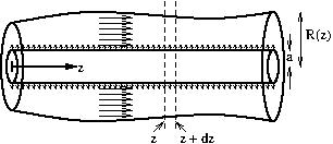
Figure 6.42. Wavy-walled pipe – planes to apply mass conservation.
The volumetric flux into the left-hand surface of this region equals area times velocity:
\begin{equation*} \pi (R^2-a^2)u \end{equation*}
and that out of the right-hand surface equals
\begin{equation*} \pi \left((R+\de R)^2-a^2\right)(u+\de u) =\pi \left(\left(R+R'\de z\right)^2-a^2\right)\left(u+u'\de z\right), \end{equation*}
where we used the chain rule to rewrite the increments in terms of \(\de z\text{.}\) Note that throughout this equation, we neglect \(\de z^2\) and higher powers, as they are small.
6.11.3.b
Solution.
The area of the inner cylinder in this region is \(2\pi a\de z\text{,}\) and thus we have a volumetric flux \(2\pi aU\de z\) entering this region from the inner cylinder.
6.11.3.c
Solution.
Since the volume of the pipe between \(z\) and \(z+\de z\) is fixed, the total volumetric flux into this region equals the total volumetric flux out.
Thus
\begin{align*} &\pi (R^2-a^2)u + 2\pi aU\de z = \pi \left(\left(R+R'\de z\right)^2-a^2\right)\left(u+u'\de z\right),\\ \Rightarrow\quad& 2\pi aU\de z = \pi \left((R^2-a^2)u'+2RR'u\right)\de z,\\ \Rightarrow\quad& 2aU = (R^2-a^2)u'+2RR'u,\\ \Rightarrow\quad& u' = \frac{2(aU-RR'u)}{R^2-a^2}, \end{align*}
thus proving the result.
6.11.3.d
Solution.
A suitable lengthscale is \(R_0\text{.}\) Simplifying the differential equation for \(u\text{,}\) by neglecting variations in pipe radius \(R'\) and the radius of the inner cylinder \(a\text{,}\) gives
\begin{equation*} \dd{u}{z} \approx \frac{2aU}{R_0^2}, \end{equation*}
suggesting a suitable velocity scale is this times \(L\) (the velocity that would be attained at the end of the pipe):
\begin{equation*} \frac{2aLU}{R_0^2}. \end{equation*}
Hence the Reynolds number is
\begin{equation*} \mathrm{Re}=\frac{\rho R_0}{\mu}\frac{2aLU}{R_0^2} =\frac{2aLU\rho}{\mu R_0}. \end{equation*}
Many students did not find an expression for the velocity scale, and just left it as \(u(z)\) or similar. This would mean that we do not have an expression for the Reynolds number in terms of the problem parameters. Also, many students did not approximate \(R-a\) as \(R_0\text{,}\) which simplifies the expression (some did get \(R_0-a\text{,}\) but you can go further than this).
I have added a final sentence to the question to clarify that the answer should be in terms of the problem parameters as very few students attempted to find an order of magnitude for \(u(z)\text{.}\)
6.11.3.e
Solution.
The Reynolds number would need to be large (but not so large that the flow becomes turbulent).
In the limit of large Reynolds number, we would recover the Euler equation from the Navier–Stokes equation (see ExerciseΒ 6.9.11). In this limit we only need a no-penetration condition (\(\bu\cdot\hat{\bn}=0\)) and not the full no-slip conditions (\(\bu=\bzero\)), and so in this case uniform flow is possible.
6.11.3.f
Solution.
The flow would need to satisfy the no-slip boundary condition at the outer cylinder and the velocity there would therefore tend to zero.